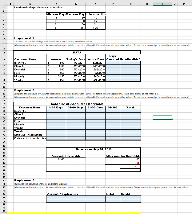
So my problem is im not really good at this excel stuff they want us to use cell refs and all that but i can never get that to work an the teacher really isnt helping people out with how to use excel for this stuff.

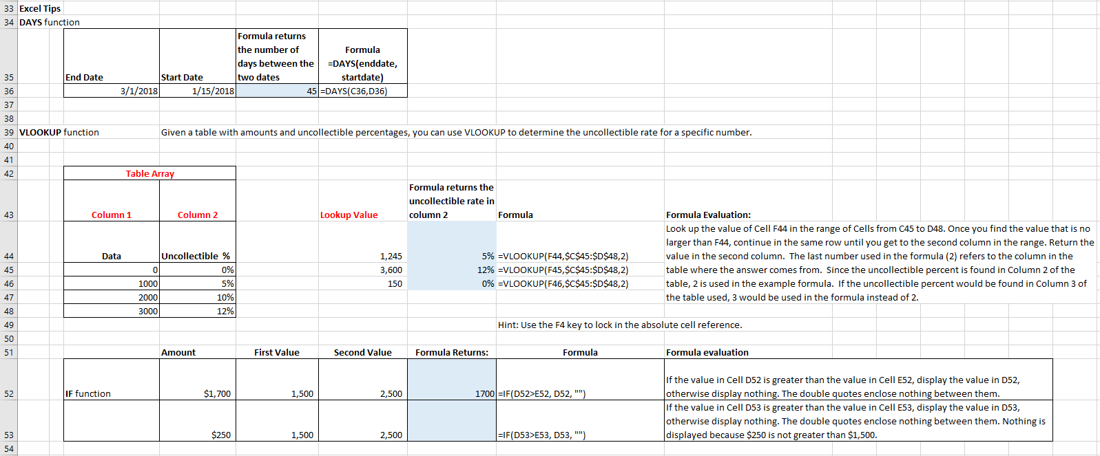
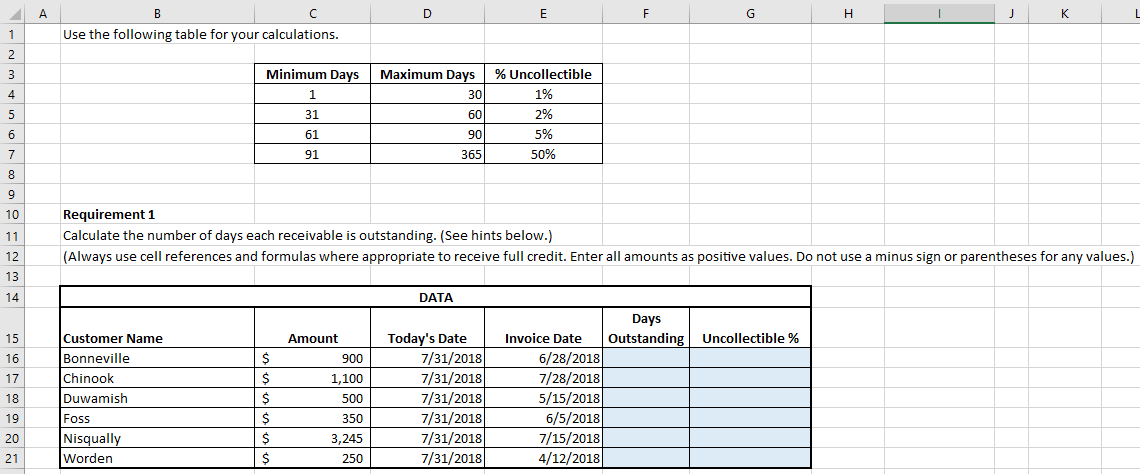
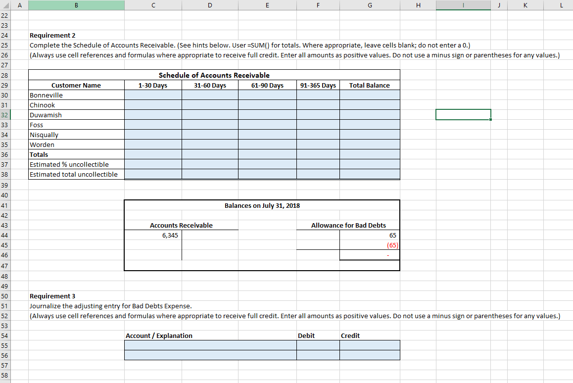
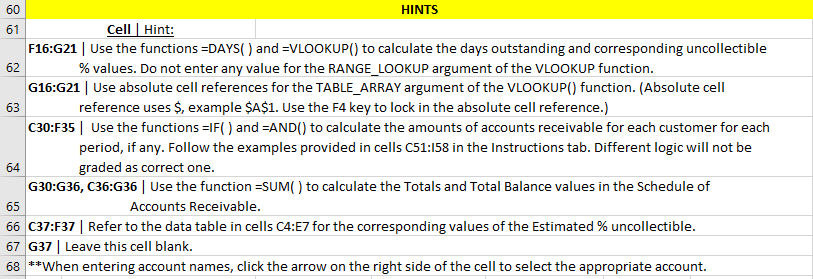
1 Receivables 2 Using Excel for Aging Accounts Receivable 4 The Lake Lucerne Company uses the allowance method of estimating bad debts expense. An aging schedule is prepared in order to calculate the balance in the allowance account. 5 The percentage uncollectible is calculated as follows: 6 1-30 Days 31-60 Days 61-90 Days 91-365 Days 1 % 7 2% 8 5% 9 50% 10 After 365 days, the account is written off. 11 12 Use the blue shaded areas on the ENTER-ANSWERS tab for inputs. 13 ALWAYS use cell references and formulas where appropriate to receive full credit. Copy/pasting values will NOT earn full points. 14 14 15 16 Requirements 17 1 Calculate the number of days each receivable is outstanding. 18. 2 Complete the Schedule of Accounts Receivable. 19 3 Journalize the adjusting entry for Bad Debts Expense. |*For all requirements, enter all amounts as positive values. Do not use a minus sign or parentheses for any values. 20 n O co 23 Excel Skills 1 Use the DAYS function to calculate the number of days between the invoice date and the date of the aging schedule. 24 2 Use the VLOOKUP function to provide the uncollectible accounts percentage based on the days outstanding. 25 3 Use IF and AND functions to determine in which column of the Accounts Receivable Schedule to place the amount for each customer. 26 4 Format cells using number and percentage formats. 27 5 Use formulas to calculate totals. 28 6 Use the Increase Indent button to indent the credit account for the journal entry. 29 7 Use Absolute references to refer to a table in the VLOOKUP formula. 30 33 Excel Tips 34 DAYS function Formula returns the number of days between the two dates Formula =DAYS(enddate, End Date Start Date startdate) 35 3/1/2018 1/15/2018 45 DAYS(C36, D36) 36 37 38 Given a table with amounts and uncollectible percentages, you can use VL0OKUP to determine the uncollectible rate for a specific number 39 VLOOKUP function 40 41 Table Array 42 Formula returns the uncollectible rate in Formula Column 1 Column 2 Lookup Value column 2 Formula Evaluation: 43 Look up the value of Cell F44 in the range of Cells from C45 to D48. Once you find the value that is no larger than F44, continue in the same row until you get to the second column in the range. Return the Uncollectible % 5% =VLOOKUP(F44,$C$45:$D$48,2) 12% =VLOOKUP (F45,$C$45:$D$48,2) 0% =VLOOKUP(F46, $C$45:$D$48,2) value in the second column. The last number used in the formula (2) refers to the column in the 44 Data 1,245 0% table where the answer comes from. Since the uncollectible percent is found in Column 2 of the 45 0 3,600 1000 5% table, 2 is used in the example formula. If the uncollectible percent would be found in Column 3 of 46 150 2000 10% the table used, 3 would be used in the formula instead of 2. 47 12% 48 3000 Hint: Use the F4 key to lock in the absolute cell reference. 49 50 Formula evaluation Second Value First Value Formula Returns: Formula 51 Amount If the value in Cell D52 is greater than the value in Cell E52, display the value in D52, otherwise display nothing. The double quotes enclose nothing between them If the value in Cell D53 is greater than the value in Cell E53, display the value in D53, otherwise display nothing. The double quotes enclose nothing between them. Nothing is displayed because $250 is not greater than $1,500. IF function 1700 F(D52>E52, D52, "") $1,700 52 1,500 2,500 =IF(D53>E53, D53, "") $250 1,500 53 2,500 54 55 6 Formula 61-90 Days Formula Returns: 31-60 Days 57 31-60 Days 61-90 Days Amount Days IF and AND functions =IF(AND(E58-31, E58=31, E5961, E58 61 and E58-31 and ES9 61 and E59E52, D52, "") $1,700 52 1,500 2,500 =IF(D53>E53, D53, "") $250 1,500 53 2,500 54 55 6 Formula 61-90 Days Formula Returns: 31-60 Days 57 31-60 Days 61-90 Days Amount Days IF and AND functions =IF(AND(E58-31, E58=31, E5961, E58 61 and E58-31 and ES9 61 and E59