solve and calculate the following questions thank you

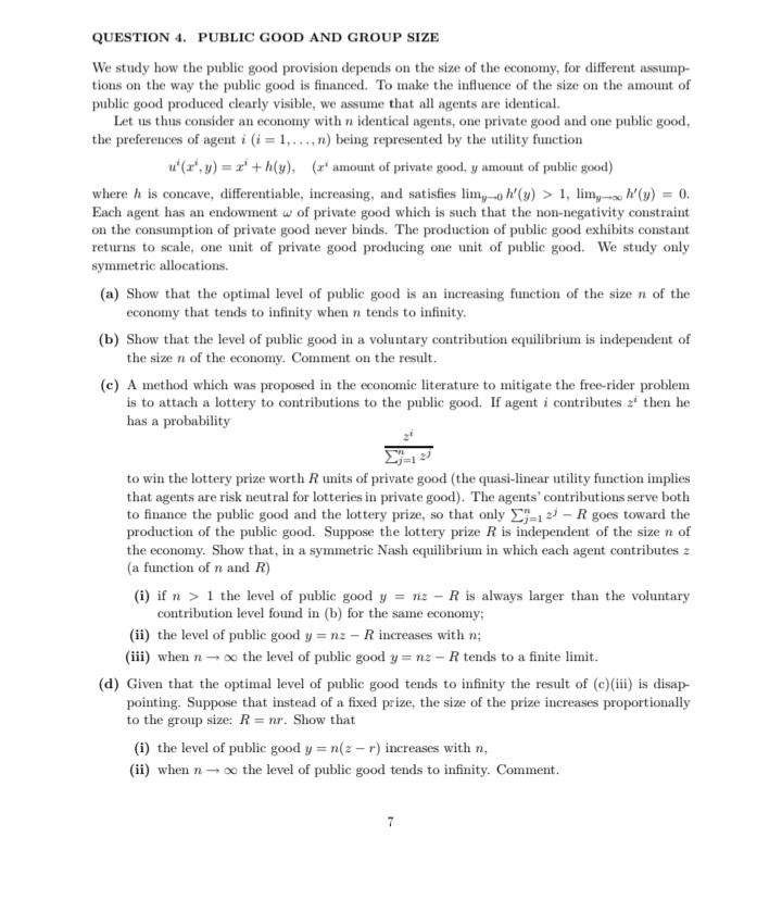
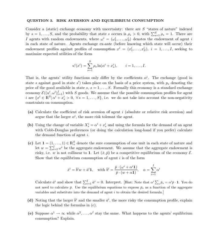
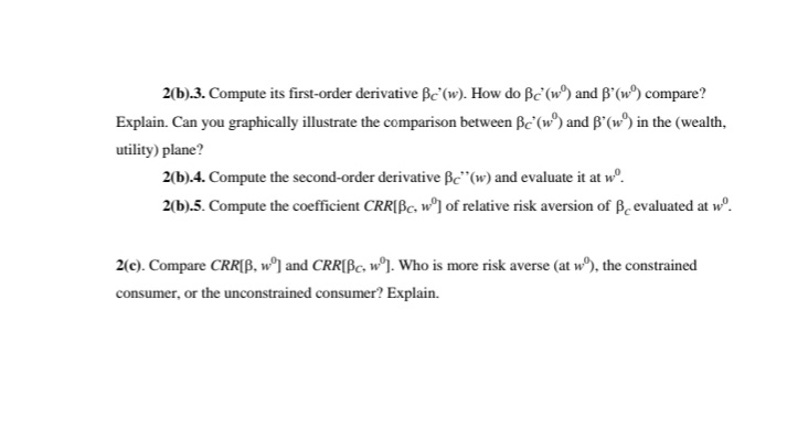
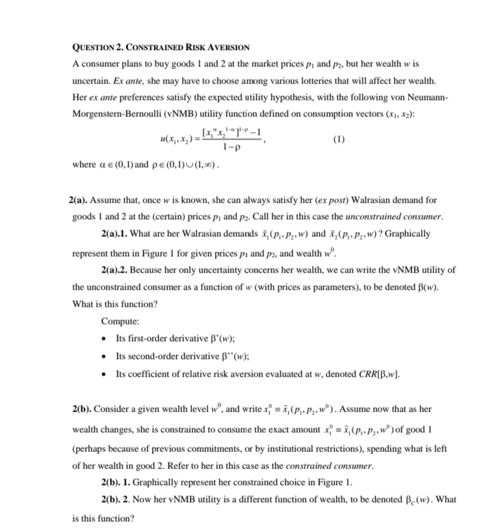
QUESTION 4. PUBLIC GOOD AND GROUP SIZE We study how the public good provision depends on the size of the economy, for different assump- tions on the way the public good is financed. To make the influence of the size on the amount of public good produced clearly visible, we assume that all agents are identical. Let us thus consider an economy with n identical agents, one private good and one public good, the preferences of agent i (i = 1, ..., n) being represented by the utility function u'(r',y) = r' +h(y), (r amount of private good, y amount of public good) where h is concave, differentiable, increasing, and satisfies limy ch'(y) > 1, lim,- h'(y) = 0. Each agent has an endowment w of private good which is such that the non-negativity constraint on the consumption of private good never binds. The production of public good exhibits constant returns to scale, one unit of private good producing one unit of public good. We study only symmetric allocations. (a) Show that the optimal level of public good is an increasing function of the size n of the economy that tends to infinity when n tends to infinity. (b) Show that the level of public good in a voluntary contribution equilibrium is independent of the size n of the economy. Comment on the result. (c) A method which was proposed in the economic literature to mitigate the free-rider problem is to attach a lottery to contributions to the public good. If agent i contributes a' then he has a probability to win the lottery prize worth R units of private good (the quasi-linear utility function implies that agents are risk neutral for lotteries in private good). The agents' contributions serve both to finance the public good and the lottery prize, so that only _j_1 2 - R goes toward the production of the public good. Suppose the lottery prize R is independent of the size n of the economy. Show that, in a symmetric Nash equilibrium in which each agent contributes = (a function of n and R) (i) if n > 1 the level of public good y = ne - R is always larger than the voluntary contribution level found in (b) for the same economy; (ii) the level of public good y = ne - R increases with n; (iii) when n - co the level of public good y = ne - R tends to a finite limit. (d) Given that the optimal level of public good tends to infinity the result of (c)(iii) is disap pointing. Suppose that instead of a fixed prize, the size of the prize increases proportionally to the group size: R = nr. Show that (i) the level of public good y = n(2 - r) increases with n, (ii) when n - co the level of public good tends to infinity. Comment. 7QUESTION 3. RISK AVERSION AND EQUILIBRIUM CONSUMPTION Consider a (static) exchange economy with uncertainty: there are S "states of nature" indexed by s = 1, ..., S, and the probability that state s occurs is p, > 0, with )- 2s=1 Ps = 1. There are I agents with random endowments, where w = (wj,...,') denotes the endowment of agent in each state of nature. Agents exchange ex-ante (before knowing which state will occur) their endowment profiles against profiles of consumption r' = (ri, ...,r's), i = 1, ..., I, seeking to maximize expected utilities of the form u' (x') = [p,In(@' +r;), i=1,...,I. That is, the agents' utility functions only differ by the coefficients o'. The exchange (good in state s against good in state s') takes place on the basis of a price system, with p, denoting the price of the good available in state s, s = 1, ..., 5. Formally this economy is a standard exchange economy E((u', w');=1) with S goods. We assume that the possible consumption profiles for agent i are {r' E RS [ a' + r, > 0, Vs = 1,..., S}, i.e. we do not take into account the non-negativity constraints on consumption. (a) Calculate the coefficient of risk aversion of agent i (absolute or relative risk aversion) and argue that the larger o', the more risk tolerant the agent. (b) Using the change of variable X", = a' + r'; and using the formula for the demand of an agent with Cobb-Douglas preferences (or doing the calculation long-hand if you prefer) calculate the demand function of agent i. (c) Let 1 = (1, ..., 1) ER; denote the sure consumption of one unit in each state of nature and let w = Elwi be the aggregate endowment. We assume that the aggregate endowment is risky, i.e. w is not collinear to 1. Let (3, p) be a competitive equilibrium of the economy &. Show that the equilibrium consumption of agent i is of the form "' = bw ta'l, with bi - P. (@' +o'1) p . (w + al) Calculate a' and show that ,_ a' = 0. Interpret. [Hint: Note that a E, p. = a'p . 1. You do not need to calculate p. Use the equilibrium equations to express p, as a function of the aggregate variables and substitute into the demand of agent : to obtain the desired formula.] (d) Noting that the larger b' and the smaller a', the more risky the consumption profile, explain the logic behind the formulas in (c). (e) Suppose al - co while a', ..., stay the same. What happens to the agents' equilibrium consumption? Explain.2(b).3. Compute its first-order derivative Bc'(w). How do Bc' (w ) and B'(w) compare? Explain. Can you graphically illustrate the comparison between Bc'(w ) and B'(w ) in the (wealth, utility) plane? 2(b).4. Compute the second-order derivative Bc"(w) and evaluate it at w. 2(b).5. Compute the coefficient CRR[Bc, w"] of relative risk aversion of B evaluated at w. 2(c). Compare CRR[B, w ] and CRR[Bc. w ]. Who is more risk averse (at w ), the constrained consumer, or the unconstrained consumer? Explain.QUESTION 2. CONSTRAINED RISK AVERSION A consumer plans to buy goods 1 and 2 at the market prices p, and pz, but her wealth w is uncertain. Ex ante, she may have to choose among various lotteries that will affect her wealth. Her ex ante preferences satisfy the expected utility hypothesis, with the following von Neumann- Morgenstern-Bernoulli (vNMB) utility function defined on consumption vectors (x1, x2): u(x,.X, ) = X x -1 (1) 1-p where a e (0, 1) and pe (0,1) (1,0). 2(a). Assume that, once w is known, she can always satisfy her (ex post) Walrasian demand for goods 1 and 2 at the (certain) prices p, and pz. Call her in this case the unconstrained consumer. 2(a).1. What are her Walrasian demands &, (p. p,. w) and &, (p. p, , w)? Graphically represent them in Figure 1 for given prices p, and pz, and wealth w. 2(a).2. Because her only uncertainty concerns her wealth, we can write the vNMB utility of the unconstrained consumer as a function of w (with prices as parameters), to be denoted B(w). What is this function? Compute: . Its first-order derivative B'(w); Its second-order derivative B"(w); Its coefficient of relative risk aversion evaluated at w, denoted CRR[B,w]. 2(b). Consider a given wealth level wa, and write x, = X, (p,. P2,w.). Assume now that as her wealth changes, she is constrained to consume the exact amount x, = x, (p,. p2, w") of good 1 (perhaps because of previous commitments, or by institutional restrictions), spending what is left of her wealth in good 2. Refer to her in this case as the constrained consumer. 2(b). 1. Graphically represent her constrained choice in Figure 1. 2(b). 2. Now her vNMB utility is a different function of wealth, to be denoted Be(w). What is this function