Question: solve these problems A binary communication channel transmits a sequence of bits (0s and 1s). Suppose that for any particular bit transmitted, there is a
solve these problems

![transmission is within 50 of the number of errors in the second?]n](https://dsd5zvtm8ll6.cloudfront.net/si.experts.images/questions/2024/10/6703ed49ca425_6016703ed4994ff2.jpg)
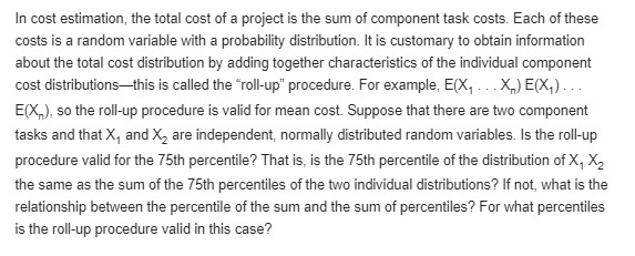
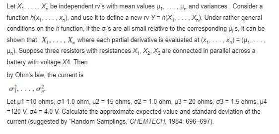
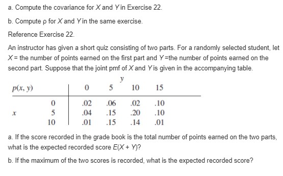
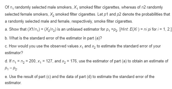
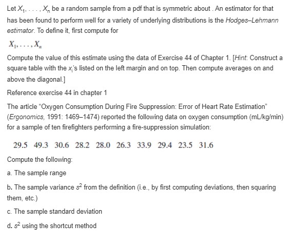
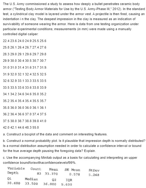
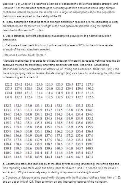
A binary communication channel transmits a sequence of "bits" (0s and 1s). Suppose that for any particular bit transmitted, there is a 10% chance of a transmission error (a 0 becoming a 1 or a 1 becoming a 0). Assume that bit errors occur independently of one another. a. Consider transmitting 1000 bits. What is the approximate probability that at most 125 transmission errors occur? b. Suppose the same 1000-bit message is sent two different times independently of one another. What is the approximate probability that the number of errors in the first transmission is within 50 of the number of errors in the second?]n cost estimation, the total cost of a project is the sum of component task costs. Each of these costs is a random variable 1.vith a proba bilitt.r distribution. It is customary to obtain information about the total cost distribution by adding together characteristics of the individual component cost distributionsthis is called the \"rollup" procedure. For example, ELK.I . . . X") EIIXIJ . . . Ean}. so the rollup procedure is valid for mean cost. Suppose that there are two component tasks and that X1 and K2 are independent: nonnallv distributed random variables. ls the rollup procedure valid for the ?5ti1 percentile? That is: is the Tth percentile of the distribution of X1 X2 the same as the sum of the E'Eth percentiles of the two individual distributions? If not what is the relationship between the percentile of the sum and the sum of percentiles? For vwrat percentiles is the rollup procedure valid in this case? Let X,, . .. . X, be independent rv's with mean values p., ..., J. and variances . Consider a function h(x,, . . ., x ), and use it to define a new rv Y = h(X, .. ., X ). Under rather general conditions on the / function, if the o's are all small relative to the corresponding p;'s, it can be shown that X. .. .. X where each partial derivative is evaluated at (x, , . . ., x ) = (H, . . . . u ). Suppose three resistors with resistances X,, X, X, are connected in parallel across a battery with voltage X4. Then by Ohm's law, the current is of. . . ..02. Let p1 =10 ohms, 01 1.0 ohm, p2 = 15 ohms, 02 = 1.0 ohm, p3 = 20 ohms, 03 = 1.5 ohms, u4 =120 V, 04 = 4.0 V. Calculate the approximate expected value and standard deviation of the current (suggested by "Random Samplings,"CHEMTECH, 1984: 696-697).a. Compute the covariance for X and Y in Exercise 22. b. Compute p for X and Yin the same exercise. Reference Exercise 22. An instructor has given a short quiz consisting of two parts. For a randomly selected student, let X = the number of points earned on the first part and Y=the number of points earned on the second part. Suppose that the joint pmf of X and Yis given in the accompanying table. p(x, y) 0 5 10 15 .02 .06 .02 .10 X .04 .15 20 .10 10 01 .15 .14 .01 a. If the score recorded in the grade book is the total number of points earned on the two parts, what is the expected recorded score E(X + Y)? b. If the maximum of the two scores is recorded, what is the expected recorded score?Of n, randomly selected male smokers, X, smoked filter cigarettes, whereas of n2 randomly selected female smokers, X, smoked filter cigarettes. Let p1 and p2 denote the probabilities that a randomly selected male and female, respectively, smoke filter cigarettes. a. Show that (X1,) = (X,-) is an unbiased estimator for p, =p2. [Hint: E(Xi ) = ni pi for i = 1, 2.] b. What is the standard error of the estimator in part (a)? c. How would you use the observed values x, and x, to estimate the standard error of your estimator? d. If n, = n, = 200, x, = 127, and x, = 176, use the estimator of part (a) to obtain an estimate of P1 - P2. e. Use the result of part (c) and the data of part (d) to estimate the standard error of the estimator.Let Xy, .. .. X be a random sample from a pdf that is symmetric about . An estimator for that has been found to perform well for a variety of underlying distributions is the Hodges-Lehmann estimator. To define it, first compute for X1. . . . . X Compute the value of this estimate using the data of Exercise 44 of Chapter 1. [Hint. Construct a square table with the x's listed on the left margin and on top. Then compute averages on and above the diagonal.] Reference exercise 44 in chapter 1 The article "Oxygen Consumption During Fire Suppression: Error of Heart Rate Estimation" (Ergonomics, 1991: 1469-1474) reported the following data on oxygen consumption (mL/kg/min) for a sample of ten firefighters performing a fire-suppression simulation: 29.5 49.3 30.6 28.2 28.0 26.3 33.9 29.4 23.5 31.6 Compute the following: a. The sample range b. The sample variance s from the definition (i.e., by first computing deviations, then squaring them, etc.) c. The sample standard deviation d. s' using the shortcut methodThe U.S. Army commissioned a study to assess how deeply a bullet penetrates ceramic body armor ( Testing Body Armor Materials for Use by the U.S. Army-Phase III, 2012). In the standard test, a cylindrical clay model is layered under the armor vest. A projectile is then fired, causing an indentation in the clay. The deepest impression in the clay is measured as an indication of survivability of someone wearing the armor. Here is data from one testing organization under particular experimental conditions; measurements (in mm) were made using a manually controlled digital caliper: 22.4 23.6 24.0 24.9 25.5 25.6 25.8 26.1 26.4 26.7 27.4 27.6 28.3 29.0 29.1 29.6 29.7 29.8 29.9 30.0 30.4 30.5 30.7 30.7 31.0 31.0 31.4 31.6 31.7 31.9. 31.9 32.0 32.1 32.4 32.5 32.5 32.6 32.9 33.1 33.3 33.5 33.5 33.5 33.5 33.6 33.6 33.8 33.9 34.1 34.2 34.6 34.6 35.0 35.2 35.2 35.4 35.4 35.4 35.5 35.7 35.8 36.0 36.0 36.0 36.1 36.1 36.2 36.4 36.6 37.0 37.4 37.5 37.5 38.0 38.7 38.8 39.8 41.0 42.0 42.1 44.6 48.3 55.0 a. Construct a boxplot of the data and comment on interesting features. b. Construct a normal probability plot. Is it plausible that impression depth is normally distributed? Is a normal distribution assumption needed in order to calculate a confidence interval or bound for the true average depth pausing the foregoing data? Explain. c. Use the accompanying Minitab output as a basis for calculating and interpreting an upper confidence boundforiswithaconfidencelevelof99% Variable Count Mean SE Mean StDev Depth 83 33.370 0.578 5 . 268 Q1 Median 03 IOR 30. 400 33.500 36.000 5.600Exercise 13 of Chapter 1 presented a sample of observations on ultimate tensile strength, and Exercise 17 of the previous section gave summary quantities and requested a large-sample confidence interval. Because the sample size is large, no assumptions about the population distribution are required for the validity of the CI. 3. Is any assumption about the tensile-strength distribution required prior to calculating a lower prediction bound for the tensile strength of the next specimen selected using the method described in this section? Explain. b. Use a statistical software package to investigate the plausibility of a normal population distribution. c. Calculate a lower prediction bound with a prediction level of 95%% for the ultimate tensile strength of the next specimen selected. Reference Exercise 13 of Chapter 1 Allowable mechanical properties for structural design of metallic aerospace vehicles requires an approved method for statistically analyzing empirical test data. The article "Establishing Mechanical Property Allowables for Metals" (J. of Testing and Evaluation, 1098: 203-290) used the accompanying data on tensile ultimate strength (ksi) as a basis for addressing the difficulties in developing such a method. 122.2 124.2 124.3 125.6 126.3 126.5 126.5 127.2 127.3 127.5 127.9 128.6 128.8 129.0 129.2 129.4 129.6 130.2 130.4 130.8 131.3 131.4 131.4 131.5 131.6 131.6 131.8 131.8 132.3 132.4 1324 132.5 132.5 132.5 132.5 132.6 132.7 132.9 133.0 133.1 133.1 133.1 133.1 133.2 133.2 133.2 133.3 133.3 133.5 1335 133.5 133.8 133.9 134.0 134.0 134.0 134.0 134.1 134.2 134.3 134.4 134.4 134.6 134.7 134.7 134.7 134.8 134.8 134.8 134.9 134.9 135.2 135.2 135.2 135.3 135.3 1354 135.5 135.5 135.6 135.6 135.7 135.8 135.8 135.8 135.8 135.8 135.9 135.9 135.9 135.9 136.0 136.0 136.1 136.2 136.2 136.3 136.4 136.4 136.6 136.8 136.9 136.9 137.0 137.1 137.2 137.6 137.6 137.8 137.8 137.8 137.9 137.9 138.2 138.2 1383 138.3 138.4 1384 138.4 138.5 138.5 138.6 138.7 138.7 139.0 139.1 139.5 139.6 139.8 139.8 140.0 140.0 140.7 140.7 140.9 140.9 141.2 141.4 141.5 141.6 142.9 143.4 143.5 143.6 143.8 143.8 143.9 144.1 1445 1445 147.7 147.7 a. Construct a stem-and-leaf display of the data by first deleting (truncating) the tenths digit and then repeating each stem value five times (once for leaves 1 and 2, a second time for leaves 3 and 4, etc.). Why is it relatively easy to identify a representative strength value? b. Construct a histogram using equal-width classes with the first class having a lower limit of 122 and an upper limit of 124. Then comment on any interesting features of the histogram.Let X1, X2 .......) Xbe a random sample from a continuous probability distribution having median X , X2, . . . . X, a. Show that P(X; = /) = P(X; = M) = .5). b. For each of six normal male infants, the amount of the amino acid alanine (mg/100 mL) was determined while the infants were on an isoleucine-free diet, resulting in the following data: a. Show that P(min (X;) ju}. But max (X,) = p iff X; Su for all i.] Compute a 97% CI for the true median amount of alanine for infants on such a diet ("The Essential Amino Acid Requirements of Infants," Amer. J. of Nutrition, 1964: 322-330). c. Let x 2) denote the second smallest of the x.s and 2.84 3.54 2.80 1.44 2.94 2.70 denote the second largest of the X.S. What is the confidence level of the interval c. Let x2) denote the second smallest of the x,'s and X(-1) denote the second largest of the x;'s. What is the confi- dence level of the interval (X(2) *(m-1)) for u
Step by Step Solution
There are 3 Steps involved in it

Get step-by-step solutions from verified subject matter experts


