Some questions are combined so see carefully.Specify which answer is for which question!

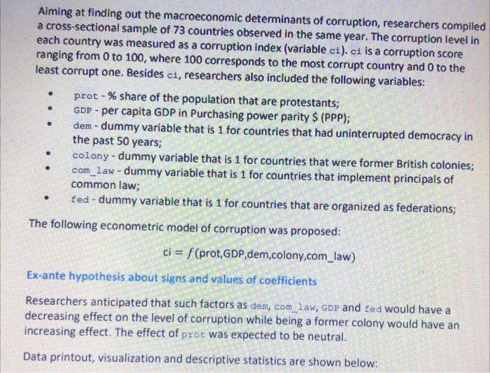
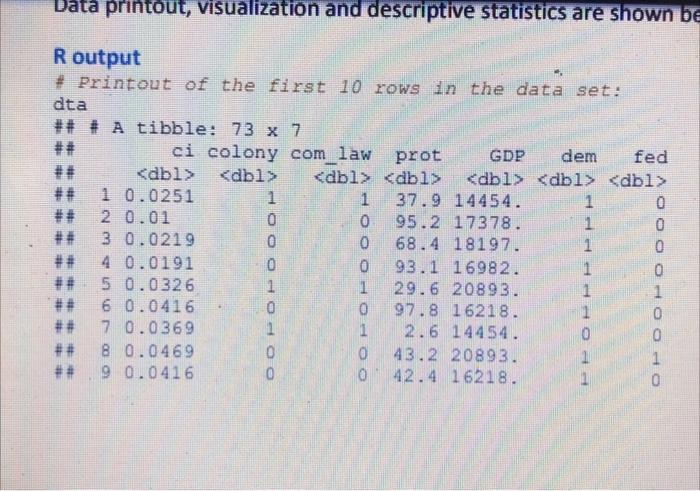
Aiming at finding out the macroeconomic determinants of corruption, researchers compiled a cross-sectional sample of 73 countries observed in the same year. The corruption level in each country was measured as a corruption index (variable ci). ci is a corruption score ranging from 0 to 100, where 100 corresponds to the most corrupt country and 0 to the least corrupt one. Besides ci, researchers also included the following variables: - . prot -% share of the population that are protestants; GDP - per capita GDP in Purchasing power parity $ (PPP); dem - dummy variable that is 1 for countries that had uninterrupted democracy in the past 50 years; colony - dummy variable that is 1 for countries that were former British colonies; com_law - dummy variable that is 1 for countries that implement principals of common law; fed - dummy variable that is 1 for countries that are organized as federations; The following econometric model of corruption was proposed: ci = f (prot,GDP,dem,colony.com_law) Ex-ante hypothesis about signs and values of coefficients Researchers anticipated that such factors as dem, com_law, GDP and fed would have a decreasing effect on the level of corruption while being a former colony would have an increasing effect. The effect of prot was expected to be neutral. Data printout, visualization and descriptive statistics are shown below: Data printout, visualization and descriptive statistics are shown be R output # Printout of the first 10 rows in the data set: dta # # # A tibble: 73 x 7 # # ci colony com_law prot GDP dem fed ##

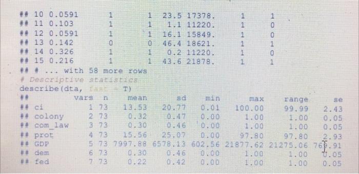
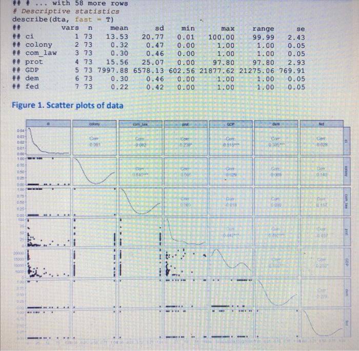
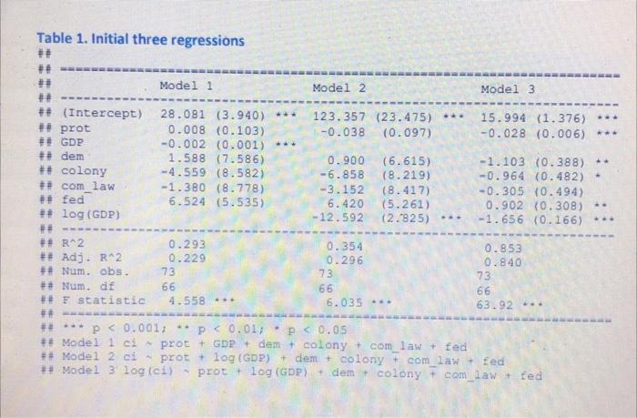
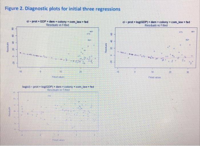
## 1 0.0251 1 1 37.9 14454. 1 0 ## 2 0.01 0 0 95.2 17378. 1 0 ## 3 0.0219 0 0 68.4 18197. 1 0 ## 4 0.0191 0 0 93.1 16982. 1 ## 5 0.0326 1 29.6 20893. 1 1 ## 6 0.0416 0 97.8 16218. 1 ## 7 0.0369 1 1 2.6 14454. 0 # # 8 0.0469 0 43.2 20893. 1 ## 9 0.0416 0 0 42.4 16218. OOOO OOOOO 0 2 EO OOO ## 10 0.0591 1 1 23.5 17378. 1 ## 11 0.103 1 1 1.1 11220. 1 ## 12 0.0591 1 1 16.1 15849. 1 ## 13 0.142 46.4 18621. 1 ## 14 0.326 1 1 0.2 11220. 1 ## 15 0.216 1 1 43.6 21878. 1 ## # ... with 58 more rows # Descriptive statistics describe (dta, T) # # vars n mean sd min max range se ## ci 173 13.53 20.77 0.01 100.00 99.99 2.43 #4 colony 273 0.32 0.47 0.00 1.00 1.00 0.05 ## com law 3 73 0.30 0.46 0.00 1.00 1.00 0.05 ++ prot 473 15.56 25.07 0.00 97.80 97.80 2.93 # GDP 5 73. 7997.88 6578.13 602.56 21877.62 21275.06 761.91 ## dem 6 73 0.30 0.46 0.00 1.00 1.00 0.05 ## fed 7.73 0.22 0.42 0.00 1.00 1.00 0.05 --- ## # with 58 more rows # Descriptive statistics describe (dta, fast - T) ## vars n mean sd min max range se # # ci 1 73 13.53 20.77 0.01 100.00 99.99 2.43 ## colony 2 73 0.32 0.47 0.00 1.00 1.00 0.05 ## com law 373 0.30 0.46 0.00 1.00 1.00 0.05 ## prot 4 73 15.56 25.07 0.00 97.80 97.80 2.93 ## GDP 5 73 7997.88 6578.13 602.56 21877.62 21275.06 769.91 ## dem 6 73 0.30 0.46 0.00 1.00 1.00 0.05 ## fed 7 73 0.22 0.42 0.00 1.00 1.00 0.05 Figure 1. Scatter plots of data COMER pro Red Can 000 Com con OST" EN 002 DO 0.00 000 Dot DOO 100 075 DO COM DO 00 100 315 CH Com Com can Cor 040 300 DO ce . . 9.00 0273 0.50 0.75 10 25 50 75 25 50 7 000 000 000 35 0.50 0 0 0 0.0 0.75 Q1. (max 10 points) Without going into any further discussions, researchers estimated three regressions (Table 1. Initial three regressions) and respective diagnostic plots (Figure 2. Diagnostic plots for initial three regressions). Below, briefly summarize the following: Why these three regressions were estimated? What are the difference between tree specifications? What goals were achieved with the Model 3 in the Table 1? Table 1. Initial three regressions ## Model 1 Model 2 Model 3 123.357 (23.475) **. -0.038 (0.097) 15.994 (1.376) +++ -0.028 (0.006) *** ## ## - # (Intercept) ++ prot #5 GDP ## dem ## colony ## com_law ## fed ## log (GDP) ## ## R2 ## Adj. R^2 ## Num. obs. # Num. df ## F statistic 28.081 (3.940) *** 0.008 (0.103) -0.002 (0.001) *** 1.588 (7.586) -4.559 (8.582) -1.380 (8.778) 6.524 (5.535) . 0.900 -6.858 -3.152 6.420 -12.592 (6.615) (8.219) (8.417) (5.261) (2.-825) -1.103 (0.388) -0.964 (0.482) -0.305 (0.494) 0.902 (0.308) -1.656 (0.166) --- 0.293 0.229 73 0.354 0.296 73 66 6.035 - 0.853 0.840 73 66 63.92 .. 66 4.558 .. - p