someone help matlab program asap thank you

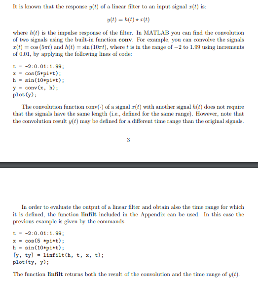
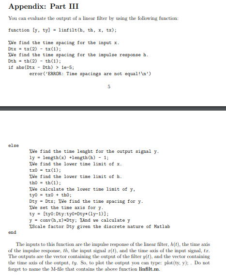
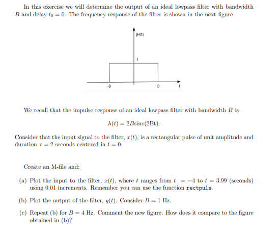
It is known that the response y(t) of a linear filter to an input signal z(t) is: y(t) = h(t)-x(t) where h(t) is the impulse response of the filter. In MATLAB you can find the convolution of two signals using the built-in function conv. For example, you can convolve the signals r(t)-cos (5t) and h(t)-sin (10t), where t is in the range of-2 to 1.99 using increments of 0.01, by applying the following lines of code t-2:0.01:1.99; x cos(5*pi*t) h = sin(10*pi*t); y conv(x, h); plot(y); The convolution functionon) of a signal (t) with another signal ht does not require that the signals have the same length (i.e., defined for the same rang). However, note that the convolution result y(t) may be defined for a different time range than the original signals. In order to evaluate the output of a linear filter and obtain also the time range for which it is defined, the function infilt included in the Appendix can be used. In this case the previous example is given by the commands: t =-2:0.01:1.99 x cos(5 *pi*t); h - sin(10*pi*t); [y, ty] -linfilt (h, t, x, t) plot(ty, y) The function linfilt returns both the result of the convolution and the time range of y(t). Appendix: Part III You can evahuate the outpu function [y, ty] linfilt(h, th, x, tx); t of a linear filter by usin g the following function: e find the time spacing for the input x Dtx-tx (2) tx (1) e find the time spacing for the impulae responseh Dth-th(2)th(1) if abs(Dtx Dth) >1e-5; error 'ERROR: Tine spacings are not equal!n) else %We find the time lenght for the output signal y ly -length(x) length (h) -1; %We find the lower time limit of X txd = tx ( 1 ) ; %We find the lower time limit of h tho th(1): %We calculate the lower time limit of y tvo-txo tho Dty-Dtx; %We find the time spacing for y %We 8et the time axis for y ty -[ty0:Dty:ty0+Dty*(ly-1)]; y-conv (h , x) *Oty; %And we calculate y %Scale factor Dty given the discrete nature of Matlab end The inputs to this function are the impulse response of the linear filter, h(t), the time axis of the impulse response, th, the input signal r(t), and the time axis of the input signal, tr. The outputs are the vector containing the output of the filter y(t), and the vector containing the time axis of the output, ty. So, to plot the output you can type: plot(ty, y); . Do not forget to name the M-file that contains the above function linfilt.m. In this exercise we will determine the output of an ideal lowpass filter with bandwidth B and delay to 0. The frequency response of the filter is shown in the next figure. HIf -B We recall that the impulse response of an ideal lowpass filter with bandwidth B is h(t)-2Bsine(2Bt). Consider that the input signal to the filter, r(t), is a rectangular pulse of unit amplitude and duration = 2 seconds centered in I = 0. Create an M-file and: (a) Plot the input to the filter, r(t), where t ranges from t =-4 to t = 3.99 (seconds) using 0.01 increments. Remember you can use the function rectpuls. (b) Plot the output of the filter, yt). Consider B 1 Hz. (c) Repeat (b) for B-4 Hz. Comment the new figure. How does it compare to the figure obtained in (b)? (d) Plot a figure with the amplitude spectrum of the filter input, |X()I. Show all spectra for f between -20 to 20 Hz (you can select this frequency range in your program with the command xlim or manually on the MATLAB plots). (e) Plot a figure with the amplitude spectra of both the filter itself |H()I for B 4 Hz and the filter output Y()l As above, show the spectra for f between -20 to 20 Hz. The amplitude spectra H(f)l and Y()I should be drawn in the same figure in a way that they are distinguishable (e.g., different type of lines). Include a legend to note which line is H()l and which is lY For that, use the Matlab command legend. Type help legend for more information. Comment the results It is known that the response y(t) of a linear filter to an input signal z(t) is: y(t) = h(t)-x(t) where h(t) is the impulse response of the filter. In MATLAB you can find the convolution of two signals using the built-in function conv. For example, you can convolve the signals r(t)-cos (5t) and h(t)-sin (10t), where t is in the range of-2 to 1.99 using increments of 0.01, by applying the following lines of code t-2:0.01:1.99; x cos(5*pi*t) h = sin(10*pi*t); y conv(x, h); plot(y); The convolution functionon) of a signal (t) with another signal ht does not require that the signals have the same length (i.e., defined for the same rang). However, note that the convolution result y(t) may be defined for a different time range than the original signals. In order to evaluate the output of a linear filter and obtain also the time range for which it is defined, the function infilt included in the Appendix can be used. In this case the previous example is given by the commands: t =-2:0.01:1.99 x cos(5 *pi*t); h - sin(10*pi*t); [y, ty] -linfilt (h, t, x, t) plot(ty, y) The function linfilt returns both the result of the convolution and the time range of y(t). Appendix: Part III You can evahuate the outpu function [y, ty] linfilt(h, th, x, tx); t of a linear filter by usin g the following function: e find the time spacing for the input x Dtx-tx (2) tx (1) e find the time spacing for the impulae responseh Dth-th(2)th(1) if abs(Dtx Dth) >1e-5; error 'ERROR: Tine spacings are not equal!n) else %We find the time lenght for the output signal y ly -length(x) length (h) -1; %We find the lower time limit of X txd = tx ( 1 ) ; %We find the lower time limit of h tho th(1): %We calculate the lower time limit of y tvo-txo tho Dty-Dtx; %We find the time spacing for y %We 8et the time axis for y ty -[ty0:Dty:ty0+Dty*(ly-1)]; y-conv (h , x) *Oty; %And we calculate y %Scale factor Dty given the discrete nature of Matlab end The inputs to this function are the impulse response of the linear filter, h(t), the time axis of the impulse response, th, the input signal r(t), and the time axis of the input signal, tr. The outputs are the vector containing the output of the filter y(t), and the vector containing the time axis of the output, ty. So, to plot the output you can type: plot(ty, y); . Do not forget to name the M-file that contains the above function linfilt.m. In this exercise we will determine the output of an ideal lowpass filter with bandwidth B and delay to 0. The frequency response of the filter is shown in the next figure. HIf -B We recall that the impulse response of an ideal lowpass filter with bandwidth B is h(t)-2Bsine(2Bt). Consider that the input signal to the filter, r(t), is a rectangular pulse of unit amplitude and duration = 2 seconds centered in I = 0. Create an M-file and: (a) Plot the input to the filter, r(t), where t ranges from t =-4 to t = 3.99 (seconds) using 0.01 increments. Remember you can use the function rectpuls. (b) Plot the output of the filter, yt). Consider B 1 Hz. (c) Repeat (b) for B-4 Hz. Comment the new figure. How does it compare to the figure obtained in (b)? (d) Plot a figure with the amplitude spectrum of the filter input, |X()I. Show all spectra for f between -20 to 20 Hz (you can select this frequency range in your program with the command xlim or manually on the MATLAB plots). (e) Plot a figure with the amplitude spectra of both the filter itself |H()I for B 4 Hz and the filter output Y()l As above, show the spectra for f between -20 to 20 Hz. The amplitude spectra H(f)l and Y()I should be drawn in the same figure in a way that they are distinguishable (e.g., different type of lines). Include a legend to note which line is H()l and which is lY For that, use the Matlab command legend. Type help legend for more information. Comment the results