someone please answer my question, this is the fourth time posting :(

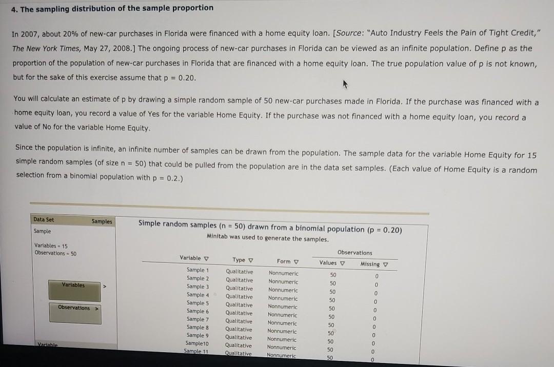
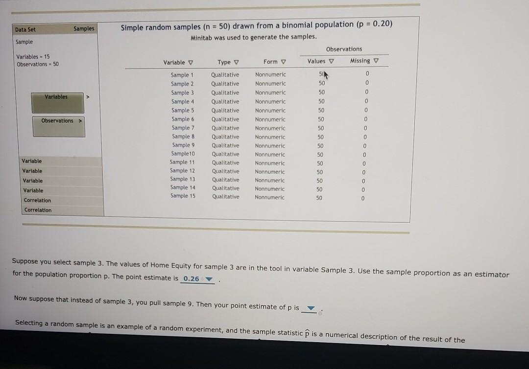
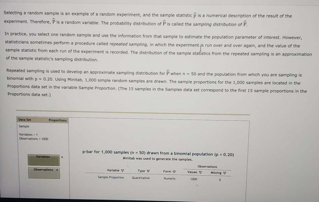
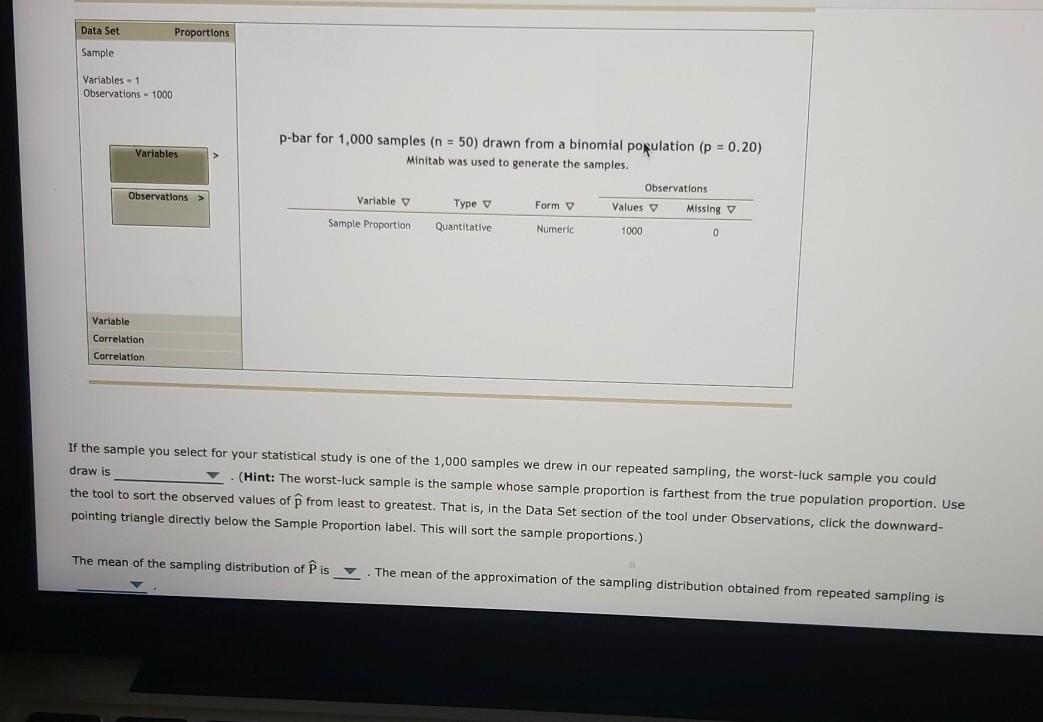
4. The sampling distribution of the sample proportion In 2007, about 20% of new-car purchases in Florida were financed with a home equity loan. [Source: "Auto Industry Feels the pain of Tight Credit," The New York Times, May 27, 2008.] The ongoing process of new-car purchases in Florida can be viewed as an infinite population. Define p as the proportion of the population of new-car purchases in Florida that are financed with a home equity loan. The true population value of p is not known, but for the sake of this exercise assume that p = 0.20. You will calculate an estimate of p by drawing a simple random sample of 50 new-car purchases made in Florida. If the purchase was financed with a home equity loan, you record a value of Yes for the variable Home Equity. If the purchase was not financed with a home equity loan, you record a value of No for the variable Home Equity. Since the population is infinite, an infinite number of samples can be drawn from the population. The sample data for the variable Home Equity for 15 simple random samples of size n = 50) that could be pulled from the population are in the data set samples. (Each value of Home Equity is a random selection from a binomial population with p = 0.2.) Data Set Samples Sample Variables = 15 Observations - 50 Variables Simple random samples (n = 50) drawn from a binomial population (p = 0.20) Minitab was used to generate the samples. Observations Variable Type v Form Values Missing Sample 1 Qualitative Nonnumeric 50 0 Sample 2 Qualitative Nonnumeric 50 0 Sample 3 Qualitative Nonnumeric 50 0 Sample 4 Qualitative Nonnumeric 50 0 Sample 5 Qualitative ancave Nonnumeric 50 0 Sample 6 Qualitative care Nonnumeric 50 0 Sample 7 Qualitative No Nonnumeric 50 0 Sample 8 Qualitative Nonnumeric 50 Sample 9 Qualitative 0 Nonnumeric 50 0 Sample 10 Qualitative Nonnumeric 50 0 Sample 11 Qualitative Nonnumeric 50 0 Observations > Non Vaciable Data Set Samples Simple random samples (n = 50) drawn from a binomial population (p = 0.20) Minitab was used to generate the samples. Sample Variables = 15 Observations - 50 Variable v Form v Variables Sample 1 Sample 2 Sample 3 Sample 4 Sample 5 Sample 6 Sample 7 Sample 8 Sample 9 Sample 10 Sample 11 Sample 12 Sample 13 Sample 14 Sample 15 Observations > Type 0 Qualitative Qualitative Qualitative Qualitative Qualitative Qualitative Qualitative Qualitative Qualitative Qualitative Qualitative Qualitative Qualitative Qualitative Qualitative Observations Values v Missing 5 0 50 0 50 0 50 0 50 0 50 0 50 0 50 0 Nonnumeric Nonnumeric Nonnumeric Nonnumeric Nonnumeric Nonnumeric Nonnumeric Nonnumeric Nonnumeric Nonnumeric Nonnumeric Nonnumeric Nonnumeric Nonnumeric Nonnumeric 50 0 0 50 Variable 50 Variable 50 50 Variable 0 0 0 0 0 Variable 50 50 Correlation Correlation Suppose you select sample 3. The values of Home Equity for sample 3 are in the tool in variable Sample 3. Use the sample proportion as an estimator for the population proportion p. The point estimate is 0.26 Now suppose that instead of sample 3, you pull sample 9. Then your point estimate of p is Selecting a random sample is an example of a random experiment, and the sample statistic p is a numerical description of the result of the Selecting a random sample is an example of a random experiment, and the sample statistic p is a numerical description of the result of the experiment. Therefore, is a random variable. The probability distribution of is called the sampling distribution of . In practice, you select one random sample and use the information from that sample to estimate the population parameter of interest. However, statisticians sometimes perform a procedure called repeated sampling, in which the experimentis run over and over again, and the value of the sample statistic from each run of the experiment is recorded. The distribution of the sample statistics from the repeated sampling is an approximation of the sample statistic's sampling distribution. Repeated sampling is used to develop an approximate sampling distribution for when n = 50 and the population from which you are sampling is binomial with p = 0.20. Using Minitab, 1,000 simple random samples are drawn. The sample proportions for the 1,000 samples are located in the Proportions data set in the variable Sample Proportion. (The 15 samples in the Samples data set correspond to the first 15 sample proportions in the Proportions data set.) Data Set Proportions Sample Variables - 1 Observations - 1000 Variables p-bar for 1,000 samples (n = 50) drawn from a binomial population (p = 0.20) Minitab was used to generate the samples. Observations Variable v Type V Form v Values o Missing Sample Proportion Quantitative Numeric 1000 0 Observations > Data Set Proportions Sample Variables - 1 Observations - 1000 Variables p-bar for 1,000 samples (n = 50) drawn from a binomial population (p = 0.20) Minitab was used to generate the samples. Observations Variable y Type v Form Values Missing v Sample Proportion Quantitative Numeric 1000 0 Observations > Variable Correlation Correlation If the sample you select for your statistical study is one of the 1,000 samples we drew in our repeated sampling, the worst-luck sample you could draw is (Hint: The worst-luck sample is the sample whose sample proportion is farthest from the true population proportion. Use the tool to sort the observed values of from least to greatest. That is, in the Data Set section of the tool under Observations, click the downward- pointing triangle directly below the Sample Proportion label. This will sort the sample proportions.) The mean of the sampling distribution of his The mean of the approximation of the sampling distribution obtained from repeated sampling is 4. The sampling distribution of the sample proportion In 2007, about 20% of new-car purchases in Florida were financed with a home equity loan. [Source: "Auto Industry Feels the pain of Tight Credit," The New York Times, May 27, 2008.] The ongoing process of new-car purchases in Florida can be viewed as an infinite population. Define p as the proportion of the population of new-car purchases in Florida that are financed with a home equity loan. The true population value of p is not known, but for the sake of this exercise assume that p = 0.20. You will calculate an estimate of p by drawing a simple random sample of 50 new-car purchases made in Florida. If the purchase was financed with a home equity loan, you record a value of Yes for the variable Home Equity. If the purchase was not financed with a home equity loan, you record a value of No for the variable Home Equity. Since the population is infinite, an infinite number of samples can be drawn from the population. The sample data for the variable Home Equity for 15 simple random samples of size n = 50) that could be pulled from the population are in the data set samples. (Each value of Home Equity is a random selection from a binomial population with p = 0.2.) Data Set Samples Sample Variables = 15 Observations - 50 Variables Simple random samples (n = 50) drawn from a binomial population (p = 0.20) Minitab was used to generate the samples. Observations Variable Type v Form Values Missing Sample 1 Qualitative Nonnumeric 50 0 Sample 2 Qualitative Nonnumeric 50 0 Sample 3 Qualitative Nonnumeric 50 0 Sample 4 Qualitative Nonnumeric 50 0 Sample 5 Qualitative ancave Nonnumeric 50 0 Sample 6 Qualitative care Nonnumeric 50 0 Sample 7 Qualitative No Nonnumeric 50 0 Sample 8 Qualitative Nonnumeric 50 Sample 9 Qualitative 0 Nonnumeric 50 0 Sample 10 Qualitative Nonnumeric 50 0 Sample 11 Qualitative Nonnumeric 50 0 Observations > Non Vaciable Data Set Samples Simple random samples (n = 50) drawn from a binomial population (p = 0.20) Minitab was used to generate the samples. Sample Variables = 15 Observations - 50 Variable v Form v Variables Sample 1 Sample 2 Sample 3 Sample 4 Sample 5 Sample 6 Sample 7 Sample 8 Sample 9 Sample 10 Sample 11 Sample 12 Sample 13 Sample 14 Sample 15 Observations > Type 0 Qualitative Qualitative Qualitative Qualitative Qualitative Qualitative Qualitative Qualitative Qualitative Qualitative Qualitative Qualitative Qualitative Qualitative Qualitative Observations Values v Missing 5 0 50 0 50 0 50 0 50 0 50 0 50 0 50 0 Nonnumeric Nonnumeric Nonnumeric Nonnumeric Nonnumeric Nonnumeric Nonnumeric Nonnumeric Nonnumeric Nonnumeric Nonnumeric Nonnumeric Nonnumeric Nonnumeric Nonnumeric 50 0 0 50 Variable 50 Variable 50 50 Variable 0 0 0 0 0 Variable 50 50 Correlation Correlation Suppose you select sample 3. The values of Home Equity for sample 3 are in the tool in variable Sample 3. Use the sample proportion as an estimator for the population proportion p. The point estimate is 0.26 Now suppose that instead of sample 3, you pull sample 9. Then your point estimate of p is Selecting a random sample is an example of a random experiment, and the sample statistic p is a numerical description of the result of the Selecting a random sample is an example of a random experiment, and the sample statistic p is a numerical description of the result of the experiment. Therefore, is a random variable. The probability distribution of is called the sampling distribution of . In practice, you select one random sample and use the information from that sample to estimate the population parameter of interest. However, statisticians sometimes perform a procedure called repeated sampling, in which the experimentis run over and over again, and the value of the sample statistic from each run of the experiment is recorded. The distribution of the sample statistics from the repeated sampling is an approximation of the sample statistic's sampling distribution. Repeated sampling is used to develop an approximate sampling distribution for when n = 50 and the population from which you are sampling is binomial with p = 0.20. Using Minitab, 1,000 simple random samples are drawn. The sample proportions for the 1,000 samples are located in the Proportions data set in the variable Sample Proportion. (The 15 samples in the Samples data set correspond to the first 15 sample proportions in the Proportions data set.) Data Set Proportions Sample Variables - 1 Observations - 1000 Variables p-bar for 1,000 samples (n = 50) drawn from a binomial population (p = 0.20) Minitab was used to generate the samples. Observations Variable v Type V Form v Values o Missing Sample Proportion Quantitative Numeric 1000 0 Observations > Data Set Proportions Sample Variables - 1 Observations - 1000 Variables p-bar for 1,000 samples (n = 50) drawn from a binomial population (p = 0.20) Minitab was used to generate the samples. Observations Variable y Type v Form Values Missing v Sample Proportion Quantitative Numeric 1000 0 Observations > Variable Correlation Correlation If the sample you select for your statistical study is one of the 1,000 samples we drew in our repeated sampling, the worst-luck sample you could draw is (Hint: The worst-luck sample is the sample whose sample proportion is farthest from the true population proportion. Use the tool to sort the observed values of from least to greatest. That is, in the Data Set section of the tool under Observations, click the downward- pointing triangle directly below the Sample Proportion label. This will sort the sample proportions.) The mean of the sampling distribution of his The mean of the approximation of the sampling distribution obtained from repeated sampling is