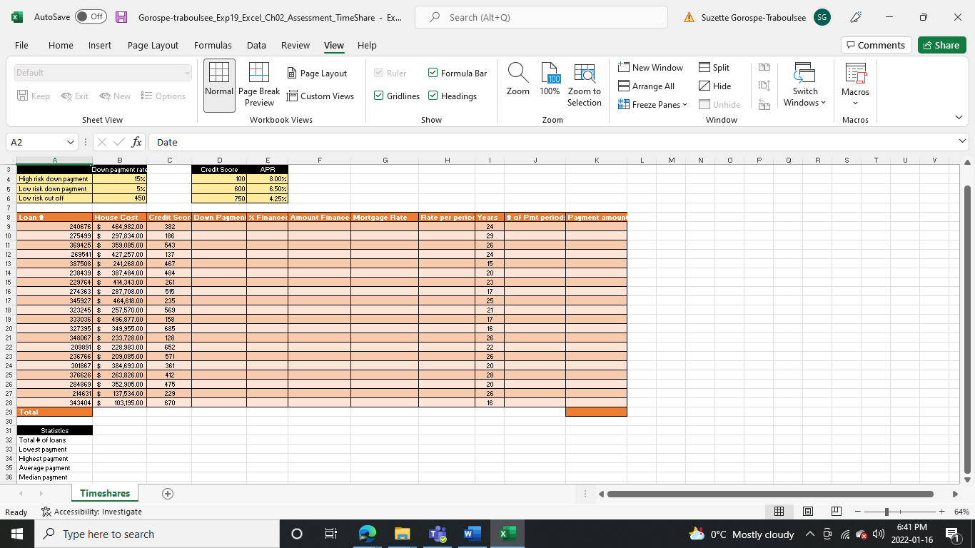
Question
Step Instructions 1 Download and open the file named Exp19_Ch02_Assessment_TimeShare.xlsx . Grader has automatically added your last name to the beginning of the filename. 2
| Step | Instructions |
| 1 | Download and open the file named Exp19_Ch02_Assessment_TimeShare.xlsx. Grader has automatically added your last name to the beginning of the filename. |
| 2 | Click cell B2, click the Formulas tab, click Date & Time in the Functions Library group. Select NOW, and then click OK to enter todays date in the cell. |
| 3 | Click cell D9. On the Formulas tab, click Logical in the Function Library group, and select IF. Type C9 in the Logical_test box, type B9*$B$4 in the Value_if_true box, and type B9*$B$5 in the Value_if_false box. Click OK, and use the fill handle to copy the contents of cell D9 down the column. Click Auto Fill Options, and click Fill Without Formatting. |
| 4 | Click cell E9, type =(B9-D9)/B9, and use the fill handle to copy the contents of cell E9 down the column. Click Auto Fill Options, and click Fill Without Formatting. |
| 5 | Click cell F9, type =B9-D9, and and press CTRL+ENTER. Use the fill handle to copy the contents of cell F9 down the column. Click Auto Fill Options, and click Fill Without Formatting. |
| 6 | Click cell G9, click Lookup & Reference in the Function Library group and select VLOOKUP. Type C9 in the Lookup_value box, type $D$4:$E$6 in the Table_array box, and type 2 in the Col_index_num box. Click OK. |
| 7 | With cell G9 selected, use the fill handle to copy the contents of cell G9 down the column, stopping at row 28. Click Auto Fill Options, and click Fill Without Formatting. With the range G9:G28 selected, on the Home tab, in the Number group, click Increase Decimal twice. |
| 8 | Click cell H9, type =G9/12, and press CTRL+ENTER Use the fill handle to copy the contents of cell H9 down the column, stopping at row 28. Click Auto Fill Options, and click Fill Without Formatting. With the range H9:H28 selected, on the Home tab, in the Number group, click Increase Decimal twice. |
| 9 | Click cell J9, type =I9*12, and press CTRL+ENTER. Use the fill handle to copy the contents of cell J9 down the column. Click Auto Fill Options, and click Fill Without Formatting. |
| 10 | Click cell K9. Click the Formulas tab, click Financial, and then click PMT. Type H9 in the rate box, J9 in the NPER box, and type -F9 in the Pv box. Click OK. |
| 11 | Use the fill handle to copy the contents of cell K9 down the column. Click Auto Fill Options, and click Fill Without Formatting. |
| 12 | Click cell K29, press ALT+=, and press ENTER. |
| 13 | Click cell B32, type =COUNT(A9:A28), and press CTRL+ENTER to calculate the total # of loans. |
| 14 | Click cell B33, type =MIN(K9:K28), and press CTRL+ENTER to calculate the lowest monthly payment. |
| 15 | Click cell B34, type =MAX(K9:K28), and press CTRL+ENTER to calculate the highest monthly payment. |
| 16 | Click cell B35, type =AVERAGE(K9:K28), and press CTRL+ENTER to calculate the average monthly payment. |
| 17 | Click cell B36, type =MEDIAN(K9:K28), and press CTRL+ENTER to calculate the median monthly payment. |
| 18 | Create a footer with your name on the left side, the sheet name code in the center, and the file name on the right side. |
| 19 | Save and close Exp19_Excel_CH02_Assessment_Timeshare.xlsx. Exit Excel and submit as directed. |

Step by Step Solution
There are 3 Steps involved in it
Step: 1

Get Instant Access to Expert-Tailored Solutions
See step-by-step solutions with expert insights and AI powered tools for academic success
Step: 2

Step: 3

Ace Your Homework with AI
Get the answers you need in no time with our AI-driven, step-by-step assistance
Get Started


