Store the Ackley Function, Griewank Function, and Bukin N 6 Function in a 2D-array which has dimensions large enough using the Python language.

Compute A_sigma = gaussian_filter(A, sigma) or A_t = S * S * ... * A (t-times).

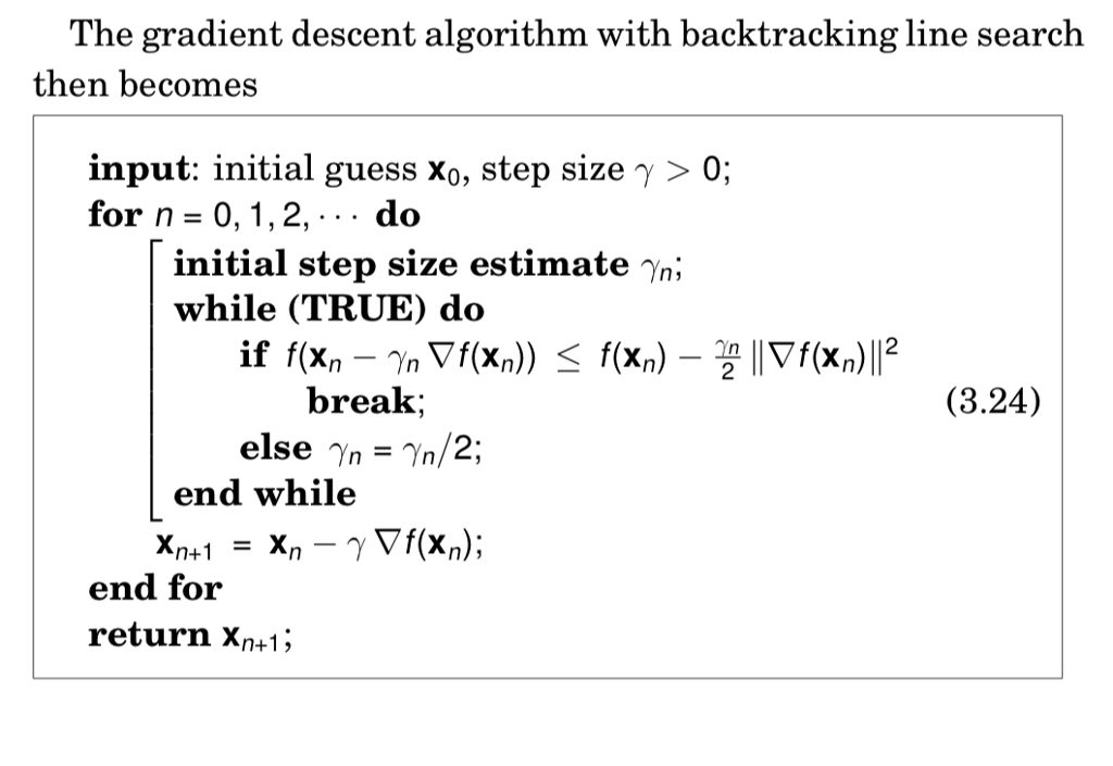
which can be considered as a convex/smooth approximation of the original function. You can use it for the estimation of f and its derivatives at x_n.. Design a set of sigma/t-values T (including "0" as the last entry) so that given an initial point x_0, the Gaussian homotopy continuation method discussed in Section 3.1.5 can locate the global minimum, while the algorithm (3.24) can find only a local minimum, for each of the functions.

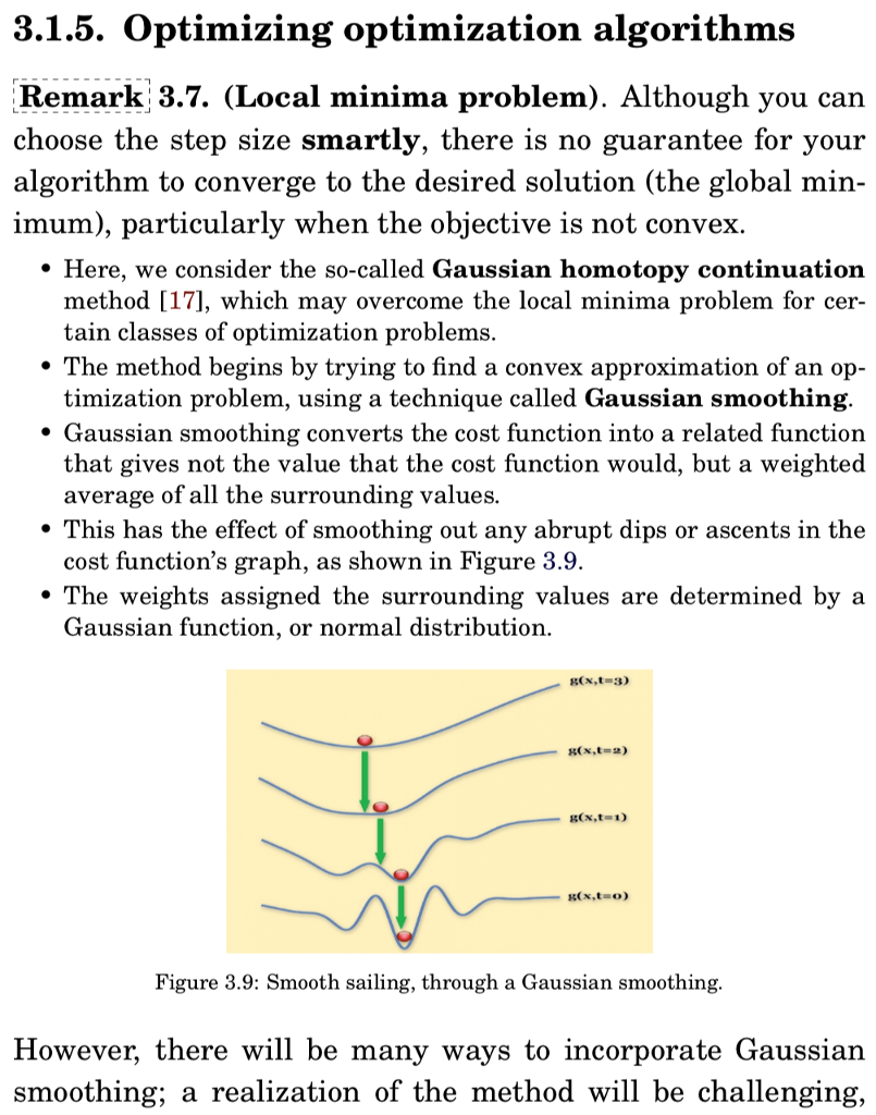
3.1.5. Optimizing optimization algorithms Remark 3.7(Local minima problem). Although you can choose the step size smartly, there is no guarantee for your algorithm to converge to the desired solution (the global min imum), particularly when the objective is not convex. * Here, we consider the so-called Gaussian homotopy continuation method [17], which may overcome the local minima problem for cer- tain classes of optimization problems. timization problem, using a technique called Gaussian smoothing that gives not the value that the cost function would, but a weighted . The method begins by trving to find a convex approximation of an op- * Gaussian smoothing converts the cost function into a related function average of all the surrounding values. cost function's graph, as shown in Figure 3.9 Gaussian function, or normal distribution * This has the effect of smoothing out any abrupt dips or ascents in the * The weights assigned the surrounding values are determined by a g(x,t 3) Cx,t 1) R(x,t o) Figure 3.9: Smooth sailing, through a Gaussian smoothing However, there will be many ways to incorporate Gaussian smoothing; a realization of the method will be challenging, 3.1.5. Optimizing optimization algorithms Remark 3.7(Local minima problem). Although you can choose the step size smartly, there is no guarantee for your algorithm to converge to the desired solution (the global min imum), particularly when the objective is not convex. * Here, we consider the so-called Gaussian homotopy continuation method [17], which may overcome the local minima problem for cer- tain classes of optimization problems. timization problem, using a technique called Gaussian smoothing that gives not the value that the cost function would, but a weighted . The method begins by trving to find a convex approximation of an op- * Gaussian smoothing converts the cost function into a related function average of all the surrounding values. cost function's graph, as shown in Figure 3.9 Gaussian function, or normal distribution * This has the effect of smoothing out any abrupt dips or ascents in the * The weights assigned the surrounding values are determined by a g(x,t 3) Cx,t 1) R(x,t o) Figure 3.9: Smooth sailing, through a Gaussian smoothing However, there will be many ways to incorporate Gaussian smoothing; a realization of the method will be challenging