streamlines and matlab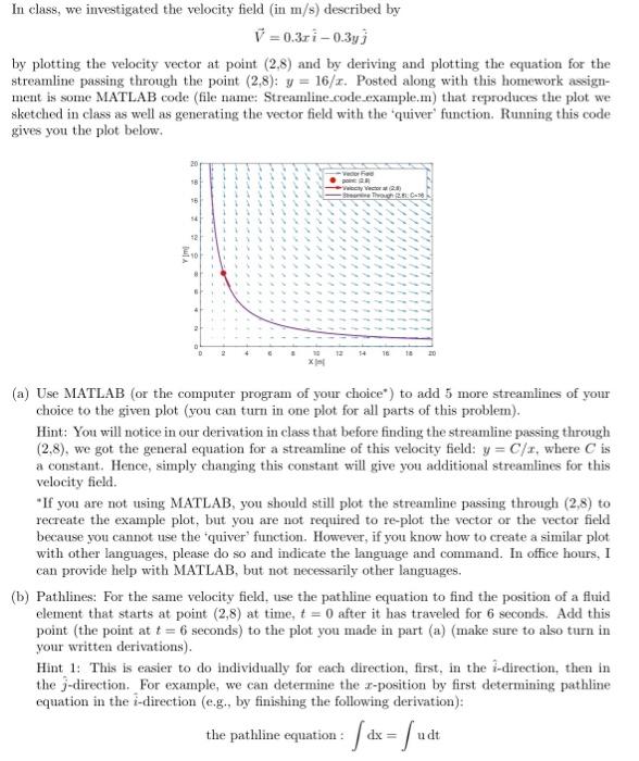

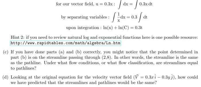
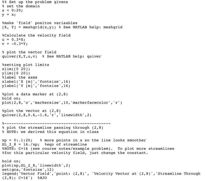
In class, we investigated the velocity field (in m/s) described by V = 0.31 i -0.3y] by plotting the velocity vector at point (2.8) and by deriving and plotting the equation for the streamline passing through the point (2,8): y = 16/x. Posted along with this homework assign- ment is some MATLAB code (file name: Streamline.code.example.m) that reproduces the plot we sketched in class as well as generating the vector field with the quiver function. Running this code gives you the plot below. 1B 12:00 56 54 42 E10 (a) Use MATLAB (or the computer program of your choice") to add 5 more streamlines of your choice to the given plot (you can turn in one plot for all parts of this problemn). Hint: You will notice in our derivation in class that before finding the streamline passing through (2.8), we got the general equation for a streamline of this velocity field: y = C/a, where C is a constant. Hence, simply changing this constant will give you additional streamlines for this velocity field. "If you are not using MATLAB, you should still plot the streamline passing through (2,8) to recreate the example plot, but you are not required to re-plot the vector or the vector field because you cannot use the quiver function. However, if you know how to create a similar plot with other languages, please do so and indicate the language and command. In office hours, I can provide help with MATLAB, but not necessarily other languages. (b) Pathlines: For the same velocity field, use the pathline equation to find the position of a fluid element that starts at point (2,8) at time, t = 0 after it has traveled for 6 seconds. Add this point (the point at t = 6 seconds) to the plot you made in part (a) (make sure to also turn in your written derivations). Hint 1: This is easier to do individually for each direction, first, in the i-direction, then in the 3-direction. For example, we can determine the 2-position by first determining pathline equation in the i-direction (e.g., by finishing the following derivation): udt the for our vector field, u = 0.3x: dx = 0.3x dt by separating variables : |dx = 0.3 dt esource: upon integration : In(x) + In(C) = 0.3t Hint 2: if you need to review natural log and exponential functions here is one possible reso http://www.rapidtables.com/math/algebra/Ln.htm (c) If you have done parts (a) and (b) correctly, you might notice that the point determined in part (b) is on the streamline passing through (2,8). In other words, the streamline is the same as the pathline. Under what flow conditions, or what flow classification, are streamlines equal to pathlines? (d) Looking at the original equation for the velocity vector field (V = 0.3c i - 0.3yj), how could we have predicted that the streamlines and pathlines would be the same? 8% Set up the problem givens $ set the domain x = 0:20; Y = x; $make 'field' positon variaables [X, Y) = meshgrid(x,y); 8 See MATLAB help: meshgrid 8Calculate the velocity field u = 0.3*X; v = -0.3*Y; % plot the vector field quiver (X, Y,u,v) | See MATLAB help: quiver $setting plot limits xlim( [0 201) ylim( [0 201) $label the axes xlabel('X [m]','fontsize',16) ylabel('Y [m]','fontsize', 16) Splot a data marker at (2,8) hold on; plot(2,8,'o', 'markersize',10,'markerfacecolor', 'r') $plot the vector at (2,8) quiver(2,8,0.6,-1.6, 'r', 'linewidth', 2) % plot the streamline passing through (2,8) % NOTE: We derived this equation in class xp = 0:.1:20; $ more points in x so the line looks smoother SL_2_8 = 16./xp; feqn of streamline NOTE: C=16 (see course notes/example problem). To plot more streamlines $for this particular velocity field, just change the constant. hold on; plot (xp, SL_2_8, 'linewidth', 2) set(gca,'fontsize', 12) legend( 'Vector Field', 'point: (2,8)', 'Velocity Vector at (2,8), 'Streamline through (2,8); C=16') HJO In class, we investigated the velocity field (in m/s) described by V = 0.31 i -0.3y] by plotting the velocity vector at point (2.8) and by deriving and plotting the equation for the streamline passing through the point (2,8): y = 16/x. Posted along with this homework assign- ment is some MATLAB code (file name: Streamline.code.example.m) that reproduces the plot we sketched in class as well as generating the vector field with the quiver function. Running this code gives you the plot below. 1B 12:00 56 54 42 E10 (a) Use MATLAB (or the computer program of your choice") to add 5 more streamlines of your choice to the given plot (you can turn in one plot for all parts of this problemn). Hint: You will notice in our derivation in class that before finding the streamline passing through (2.8), we got the general equation for a streamline of this velocity field: y = C/a, where C is a constant. Hence, simply changing this constant will give you additional streamlines for this velocity field. "If you are not using MATLAB, you should still plot the streamline passing through (2,8) to recreate the example plot, but you are not required to re-plot the vector or the vector field because you cannot use the quiver function. However, if you know how to create a similar plot with other languages, please do so and indicate the language and command. In office hours, I can provide help with MATLAB, but not necessarily other languages. (b) Pathlines: For the same velocity field, use the pathline equation to find the position of a fluid element that starts at point (2,8) at time, t = 0 after it has traveled for 6 seconds. Add this point (the point at t = 6 seconds) to the plot you made in part (a) (make sure to also turn in your written derivations). Hint 1: This is easier to do individually for each direction, first, in the i-direction, then in the 3-direction. For example, we can determine the 2-position by first determining pathline equation in the i-direction (e.g., by finishing the following derivation): udt the for our vector field, u = 0.3x: dx = 0.3x dt by separating variables : |dx = 0.3 dt esource: upon integration : In(x) + In(C) = 0.3t Hint 2: if you need to review natural log and exponential functions here is one possible reso http://www.rapidtables.com/math/algebra/Ln.htm (c) If you have done parts (a) and (b) correctly, you might notice that the point determined in part (b) is on the streamline passing through (2,8). In other words, the streamline is the same as the pathline. Under what flow conditions, or what flow classification, are streamlines equal to pathlines? (d) Looking at the original equation for the velocity vector field (V = 0.3c i - 0.3yj), how could we have predicted that the streamlines and pathlines would be the same? 8% Set up the problem givens $ set the domain x = 0:20; Y = x; $make 'field' positon variaables [X, Y) = meshgrid(x,y); 8 See MATLAB help: meshgrid 8Calculate the velocity field u = 0.3*X; v = -0.3*Y; % plot the vector field quiver (X, Y,u,v) | See MATLAB help: quiver $setting plot limits xlim( [0 201) ylim( [0 201) $label the axes xlabel('X [m]','fontsize',16) ylabel('Y [m]','fontsize', 16) Splot a data marker at (2,8) hold on; plot(2,8,'o', 'markersize',10,'markerfacecolor', 'r') $plot the vector at (2,8) quiver(2,8,0.6,-1.6, 'r', 'linewidth', 2) % plot the streamline passing through (2,8) % NOTE: We derived this equation in class xp = 0:.1:20; $ more points in x so the line looks smoother SL_2_8 = 16./xp; feqn of streamline NOTE: C=16 (see course notes/example problem). To plot more streamlines $for this particular velocity field, just change the constant. hold on; plot (xp, SL_2_8, 'linewidth', 2) set(gca,'fontsize', 12) legend( 'Vector Field', 'point: (2,8)', 'Velocity Vector at (2,8), 'Streamline through (2,8); C=16') HJO