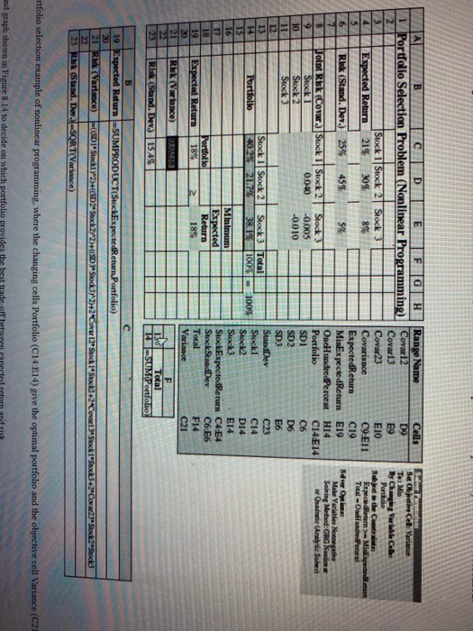
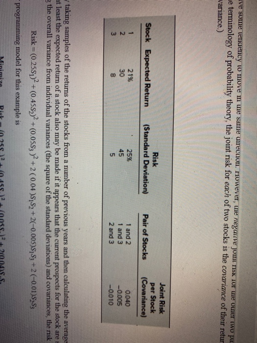
Study Pack Practice hapter 8, Problem 6P Bookmark Show all steps: ON Problem To the left of each of the following problems (or their parts), we have inserted an E' whenever Excel should be used (unless your instructor gives you contrary instructions). An asterisk on the problem number indicates that at least a partial answer is given in the back of the book. Reconsider the portfolio selection example, including its spreadsheet model in Figure 8.13, given in Section 8.2. Note in Table 8.2 that Stock 2 has the highest expected return and stock 3 has by far the lowest. Nevertheless, the changing cells Portfolio (C14:E14) provide an optimal solution that calls for purchasing far more of Stock 3 than of Stock 2. Although purchasing so much of Stock 3 greatly reduces the risk of the portfolio, an aggressive investor may be unwilling to own so much of a stock with such a low expected return. For the sake of such an investor, add a constraint to the model that specifies that the percentage of Stock 3 in the portfolio cannot exceed the amount specified by the investor. Then compare the expected return and risk (standard deviation of the return) of the optimal portfolio with that in Figure 8.13 when the upper bound on the percentage of Stock 3 allowed in the portfolio is set at the following values. a. 20% b. 0% c. Generate a parameter analysis report using RSPE to systematically try all the percentages at 5% Intervals from 0% to 50% FIGURE 8.13 A spreadsheet model for the portfolio selection example of nonlinear programming, where the changing cells Portfolio (C14:E14) give the optimal portfolio and the objective cell Variance (C21) shows the resulting risk. Portal Selection Problem anar Prering O a mo Sobre Parameter SetObjethe Ce: Variance To: Mis By Changing Variable Cele Portfolio Subject the Centres Expected earn Misspededeum Toul-Odlundredere Sdver Options Make Varles Nonethe Solving Method: GRG Nane or Quadratic Analytic Sohen B D E HFGH Range Name Cells 1 Portfolio Selection Problem (Nonlinear Programming) Covar12 D9 2 Covar 13 E9 3 Stock 1 Stock 2 Stock 3 Covar23 EIO 4 Expected Return 2156 30% 8% Covariance C9 E11 5 ExpectedReturn C19 6 Risk (Stand. Dev.) 25% 45% 5% MinExceedReturn E19 77 OncHundredPercnt HI4 8 Joint Risk (Covar.) Stock Stock 2 Stock 3 Portfolio C14 E14 9 Stock 1 0.040 -0.005 SD1 C6 10 Stock 2 -0.010 SD2 D6 11 Stock 3 SD3 12 E6 13 SundDev Stock I Stock 2 Stock 3 Total C23 Portfolio 40.2% 21.7% Stocki 100% 100% C14 15 Stock2 D14 16 Minimum Stock3 E14 11 Expected StockExpected Return C4-E4 18 Portfolio Return Stock StandDev C6:56 19 Expected Return 18% Total 18% 2 F14 20 Variance C21 21 RSK (Varlance) US F Risk (Stand. Dev.) 15.4% Total 141SUM Portfolio B 19 Expected Return =SUMPRODUCT(StockExpectedReturn Portfolio) 20 21 R Variance) =((SDI Stockly 2D2Stock272)+((SD)" Stodur 2+2 Covar 12" Stock I'Sax2+2 2 23 Risk (Stand. Dev.-SORT Variance) Stock2Stock3 rtfolio selection example of nonlinear programming, where the changing cells Portfolio (C14:E14) give the optimal portfolio and the objective cell Variance (C21 and graph shown in Figure 8.14 to decide on which portfolio provides the best trade ve some tendency to move in the same direction. However, the negative jouit nisk tor ve order iwo pa ne terminology of probability theory, the joint risk for each of two stocks is the covariance of their retur variance.) Stock Expected Return Risk (Standard Deviation) Joint Risk per Stock (Covariance) Pair of Stocks N 21% 30 8 25% 45 5 1 and 2 1 and 3 2 and 3 0.040 -0.005 -0.010 3 taking samples of the returns of the stocks from a number of previous years and then calculating the average at least the expected return of a stock also may be made if it appears that the current prospects for the stock are the overall variance from individual variances (the square of the standard deviations) and covariances, the risk Risk = (0.25%;)2 + (0.455))2 + (0.0553 )2 + 2 (0.04 )$,$2+2(-0.00598,53 +2 (-0.01)$$3 programming model for this example is 200 Study Pack Practice hapter 8, Problem 6P Bookmark Show all steps: ON Problem To the left of each of the following problems (or their parts), we have inserted an E' whenever Excel should be used (unless your instructor gives you contrary instructions). An asterisk on the problem number indicates that at least a partial answer is given in the back of the book. Reconsider the portfolio selection example, including its spreadsheet model in Figure 8.13, given in Section 8.2. Note in Table 8.2 that Stock 2 has the highest expected return and stock 3 has by far the lowest. Nevertheless, the changing cells Portfolio (C14:E14) provide an optimal solution that calls for purchasing far more of Stock 3 than of Stock 2. Although purchasing so much of Stock 3 greatly reduces the risk of the portfolio, an aggressive investor may be unwilling to own so much of a stock with such a low expected return. For the sake of such an investor, add a constraint to the model that specifies that the percentage of Stock 3 in the portfolio cannot exceed the amount specified by the investor. Then compare the expected return and risk (standard deviation of the return) of the optimal portfolio with that in Figure 8.13 when the upper bound on the percentage of Stock 3 allowed in the portfolio is set at the following values. a. 20% b. 0% c. Generate a parameter analysis report using RSPE to systematically try all the percentages at 5% Intervals from 0% to 50% FIGURE 8.13 A spreadsheet model for the portfolio selection example of nonlinear programming, where the changing cells Portfolio (C14:E14) give the optimal portfolio and the objective cell Variance (C21) shows the resulting risk. Portal Selection Problem anar Prering O a mo Sobre Parameter SetObjethe Ce: Variance To: Mis By Changing Variable Cele Portfolio Subject the Centres Expected earn Misspededeum Toul-Odlundredere Sdver Options Make Varles Nonethe Solving Method: GRG Nane or Quadratic Analytic Sohen B D E HFGH Range Name Cells 1 Portfolio Selection Problem (Nonlinear Programming) Covar12 D9 2 Covar 13 E9 3 Stock 1 Stock 2 Stock 3 Covar23 EIO 4 Expected Return 2156 30% 8% Covariance C9 E11 5 ExpectedReturn C19 6 Risk (Stand. Dev.) 25% 45% 5% MinExceedReturn E19 77 OncHundredPercnt HI4 8 Joint Risk (Covar.) Stock Stock 2 Stock 3 Portfolio C14 E14 9 Stock 1 0.040 -0.005 SD1 C6 10 Stock 2 -0.010 SD2 D6 11 Stock 3 SD3 12 E6 13 SundDev Stock I Stock 2 Stock 3 Total C23 Portfolio 40.2% 21.7% Stocki 100% 100% C14 15 Stock2 D14 16 Minimum Stock3 E14 11 Expected StockExpected Return C4-E4 18 Portfolio Return Stock StandDev C6:56 19 Expected Return 18% Total 18% 2 F14 20 Variance C21 21 RSK (Varlance) US F Risk (Stand. Dev.) 15.4% Total 141SUM Portfolio B 19 Expected Return =SUMPRODUCT(StockExpectedReturn Portfolio) 20 21 R Variance) =((SDI Stockly 2D2Stock272)+((SD)" Stodur 2+2 Covar 12" Stock I'Sax2+2 2 23 Risk (Stand. Dev.-SORT Variance) Stock2Stock3 rtfolio selection example of nonlinear programming, where the changing cells Portfolio (C14:E14) give the optimal portfolio and the objective cell Variance (C21 and graph shown in Figure 8.14 to decide on which portfolio provides the best trade ve some tendency to move in the same direction. However, the negative jouit nisk tor ve order iwo pa ne terminology of probability theory, the joint risk for each of two stocks is the covariance of their retur variance.) Stock Expected Return Risk (Standard Deviation) Joint Risk per Stock (Covariance) Pair of Stocks N 21% 30 8 25% 45 5 1 and 2 1 and 3 2 and 3 0.040 -0.005 -0.010 3 taking samples of the returns of the stocks from a number of previous years and then calculating the average at least the expected return of a stock also may be made if it appears that the current prospects for the stock are the overall variance from individual variances (the square of the standard deviations) and covariances, the risk Risk = (0.25%;)2 + (0.455))2 + (0.0553 )2 + 2 (0.04 )$,$2+2(-0.00598,53 +2 (-0.01)$$3 programming model for this example is 200