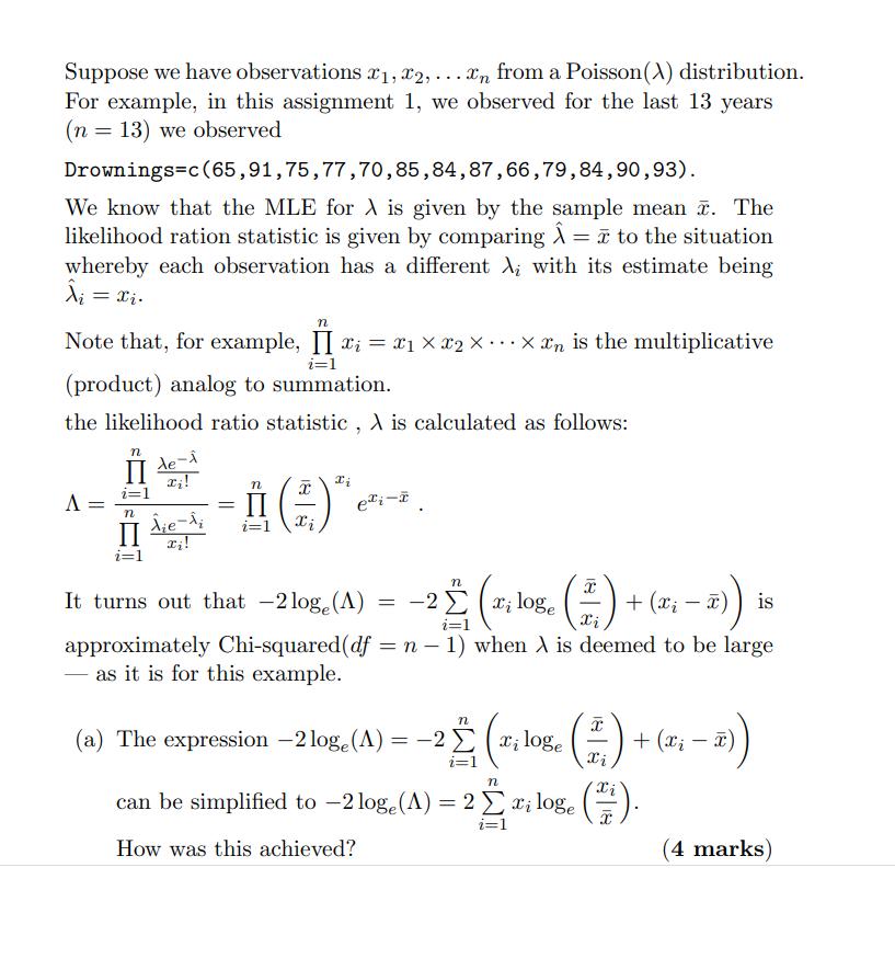
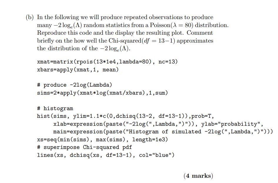
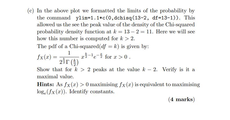
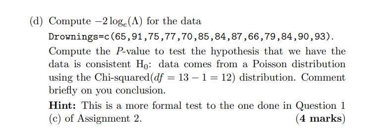
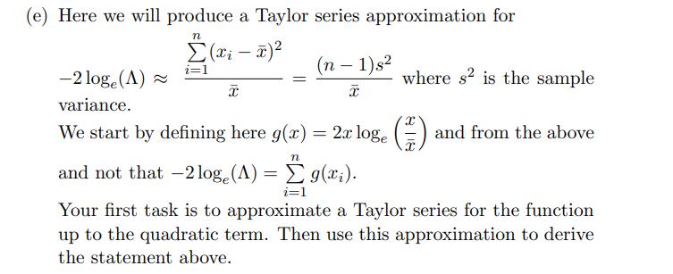
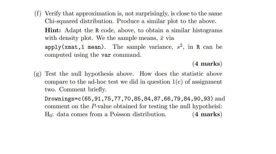
Suppose we have observations x1,x2,... n from a Poisson (X) distribution. For example, in this assignment 1, we observed for the last 13 years (n = 13) we observed Drownings c (65,91,75,77,70,85,84,87,66,79,84,90,93). We know that the MLE for A is given by the sample mean . The likelihood ration statistic is given by comparing A = to the situation whereby each observation has a different A, with its estimate being u = i n Note that, for example, II x = x2...x xn is the multiplicative x1 i=1 (product) analog to summation. the likelihood ratio statistic, A is calculated as follows: n II de-i x! i=1 A = n II i=1 e- xi! n = -A () * i= Xi ei-I It turns out that -2log (A) -22 (r; log. ()+(2-2)) is x) Xi approximately Chi-squared(df = n 1) when A is deemed to be large as it is for this example. = (a) The expression -2 loge (A) = = 22 (x log (#) + (x 2)) ( - Xi n can be simplified to - 2 loge (A) = 2 xiloge (2). i=1 How was this achieved? (4 marks) (b) In the following we will produce repeated observations to produce many -2 loge (A) random statistics from a Poisson(A = 80) distribution. Reproduce this code and the display the resulting plot. Comment briefly on the how well the Chi-squared (df = 13-1) approximates the distribution of the -2 loge (A). xmat-matrix (rpois (13*1e4, lambda=80), nc=13) xbars apply (xmat, 1, mean) # produce -2log (Lambda) sims=2*apply (xmat* log(xmat/xbars), 1, sum) # histogram hist (sims, ylim=1.1*c (0,dchisq (13-2, df=13-1)), prob=T, xlab-expression (paste ("-21og(", Lambda, ")")), ylab="probability", main=expression (paste ("Histogram of simulated -2log(", Lambda, ")"))) xs-seq (min (sims), max(sims), length=1e3) #superimpose Chi-squared pdf lines (xs, dchisq (xs, df=13-1), col="blue") (4 marks) (c) In the above plot we formatted the limits of the probability by the command ylim-1.1*c (0,dchisq (13-2, df=13-1)). This allowed us the see the peak value of the density of the Chi-squared probability density function at k = 13-211. Here we will see how this number is computed for k > 2. The pdf of a Chi-squared(df = k) is given by: 1 fx(x) = = x-e for x > 0. 2r (1) Show that for k > 2 peaks at the value k-2. Verify is it a maximal value. Hints: As fx(x) > 0 maximising fx (x) is equivalent to maximising loge (fx (x)). Identify constants. (4 marks) (d) Compute -2 loge (A) for the data Drownings c (65,91,75,77,70,85,84,87,66,79,84,90,93). Compute the P-value to test the hypothesis that we have the data is consistent Ho: data comes from a Poisson distribution using the Chi-squared (df 13 - 1 = 12) distribution. Comment briefly on you conclusion. = Hint: This is a more formal test to the one done in Question 1 (c) of Assignment 2. (4 marks) (e) Here we will produce a Taylor series approximation for n (x; - z)2 i=1 X (n-1) s X -2 loge (A) ~ variance. We start by defining here g(x) = 2x loge () and from the above n and not that -2 loge (A) = g(xi). i=1 Your first task is to approximate a Taylor series for the function up to the quadratic term. Then use this approximation to derive the statement above. = where s2 is the sample (f) Verify that approximation is, not surprisingly, is close to the same Chi-squared distribution. Produce a similar plot to the above. Hint: Adapt the R code, above, to obtain a similar histograms with density plot. We the sample means, via apply (xmat, 1 mean). The sample variance, s2, in R can be computed using the var command. (4 marks) (g) Test the null hypothesis above. How does the statistic above compare to the ad-hoc test we did in question 1(c) of assignment two. Comment briefly. Drownings c (65,91,75,77,70,85,84,87,66,79,84,90,93) and comment on the P-value obtained for testing the null hypotheisi: Ho: data comes from a Poisson distribution. (4 marks)