Suppose you have bivariate data (x1, y1), . . . ,(xn, yn). A common model is that there is a

linear relationship between x and y, so in principle the data should lie exactly along a line.

However since data has random noise and our model is probably not exact this will not be

the case. What we can do is look for the line that best fits the data. we will use

a simple linear regression model.

For bivariate data the simple linear regression model assumes that the xi are not random

but that for some values of the parameters a and b the value yi is drawn from the random

variable

Yi ? axi + b + ?i

where ?i is a normal random variable with mean 0 and variance ?2. We assume all of the

random variables ?i are independent.

Notes. 1. The model assumes that ? is a known constant, the same for each ?i.

2. We think of ?i as the measurement error, so the model says that

yi = axi + b + random measurement error.

3. Remember that (xi, yi) are not variables. They are values of data.

(a) The distribution of Yi depends on a, b, ? and xi. Of these only a and b are not known.

Give the formula for the likelihood function f(yi | a, b, xi, ?) corresponding to one random

value yi. (Hint: yi ? axi ? b ? N(0, ?2).)

(b) (i) Suppose we have data (1, 8), (3, 2), (5, 1). Based on our model write down the

likelihood and log likelihood as functions of a, b, and ?.

(ii) For general data (x1, y1), . . . ,(xn, yn) give the likelihood and and log likelihood functions

(again as functions of a, b, and ?).

(c) Assume ? is a constant, known value. For the data in part b(i) find the maximum

likelihood estimates for a and b

10. What is the relationship between correlation and least squares fit line?

11. You have bivariate data (xi, yi). You have reason to suspect the data is related by

yi = a/xi + Ui where Ui is a random variable with mean 0 and variance ?2 (the same for

all.

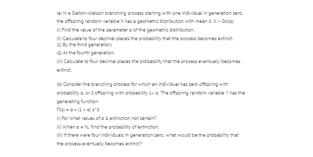
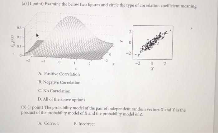
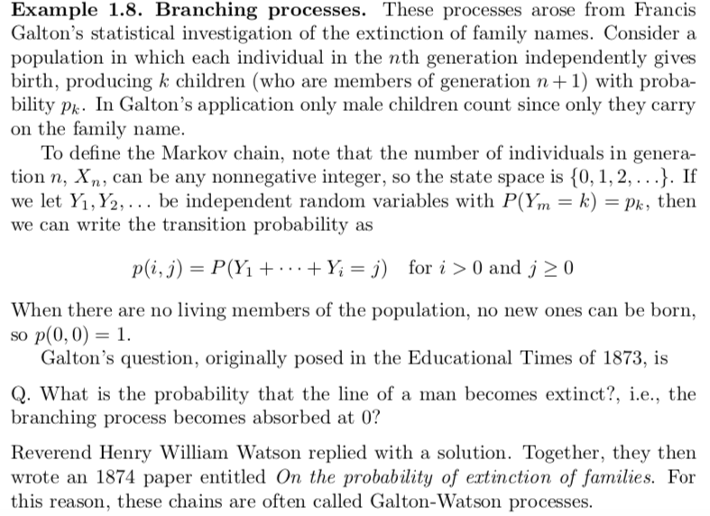
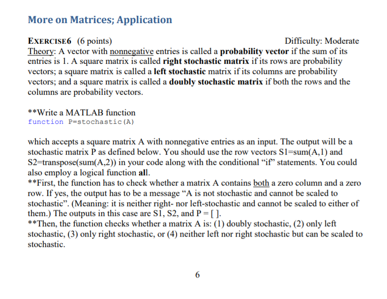
(a) (1 point) Examine the below two figures and circle the type of correlation coefficient meaning 0.3 2 0.2 0.1 -2 -2 -2 2 -2 2 Y A. Positive Correlation B. Negative Correlation C. No Correlation D. All of the above options (b) (1 point) The probability model of the pair of independent random vectors X and Y is the product of the probability model of X and the probability model of Z. A. Correct, B. IncorrectExample 1.8. Branching processes. These processes arose from Francis Galton's statistical investigation of the extinction of family names. Consider a population in which each individual in the nth generation independently gives birth, producing k children (who are members of generation n + 1) with proba- bility px. In Galton's application only male children count since only they carry on the family name. To define the Markov chain, note that the number of individuals in genera- tion n, Xn, can be any nonnegative integer, so the state space is {0, 1, 2, . . .}. If we let Y1, Y2, . .. be independent random variables with P(Ym = k) = Pk, then we can write the transition probability as p(i, j) = P(Y1 + . . . + Yi=j) for i > 0 and j 2 0 When there are no living members of the population, no new ones can be born, so p(0, 0) = 1. Galton's question, originally posed in the Educational Times of 1873, is Q. What is the probability that the line of a man becomes extinct?, i.e., the branching process becomes absorbed at 0? Reverend Henry William Watson replied with a solution. Together, they then wrote an 1874 paper entitled On the probability of extinction of families. For this reason, these chains are often called Galton-Watson processes.[a) In a Galton-Watson branching process starting with one individual in generation zero, the offspring random variable X has a geometric distribution with mean 3: X ~ Go[p]. [ Find the value of the parameter p of the geometric distribution. [in) Calculate to four decimal places the probability that the process becomes extinct: By the third generation; [2) At the fourth generation. (iii) Calculate to four decimal places the probability that the process eventually becomes extinct. (b] Consider the branching process for which an individual has zero offspring with probability a, or 3 offspring with probability 1- a. The offspring random variable Y has the generating function n(s) = a - [1 - 0] $43. [i) For what values of a is extinction not certain? [ii) When a = 36, find the probability of extinction. (iin If there were four individuals in generation zero, what would be the probability that the process eventually becomes extinct?More on Matrices; Application EXERCISE6 (6 points) Difficulty: Moderate Theory: A vector with nonnegative entries is called a probability vector if the sum of its entries is 1. A square matrix is called right stochastic matrix if its rows are probability vectors; a square matrix is called a left stochastic matrix if its columns are probability vectors; and a square matrix is called a doubly stochastic matrix if both the rows and the columns are probability vectors. **Write a MATLAB function function P=stochastic (A) which accepts a square matrix A with nonnegative entries as an input. The output will be a stochastic matrix P as defined below. You should use the row vectors S1=sum(A, 1) and S2=transpose(sum(A,2)) in your code along with the conditional "if" statements. You could also employ a logical function all. **First, the function has to check whether a matrix A contains both a zero column and a zero row. If yes, the output has to be a message "A is not stochastic and cannot be scaled to stochastic". (Meaning: it is neither right- nor left-stochastic and cannot be scaled to either of them.) The outputs in this case are S1, S2, and P = [ ]. **Then, the function checks whether a matrix A is: (1) doubly stochastic, (2) only left stochastic, (3) only right stochastic, or (4) neither left nor right stochastic but can be scaled to stochastic. 6