Answered step by step
Verified Expert Solution
Question
1 Approved Answer
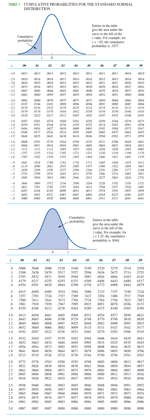
TABLE 1 CUMULATIVE PROBABILITIES FOR THE STANDARD NORMAL DISTRIBUTION Cumulative probability Entries in the table give the area under the curve to the left


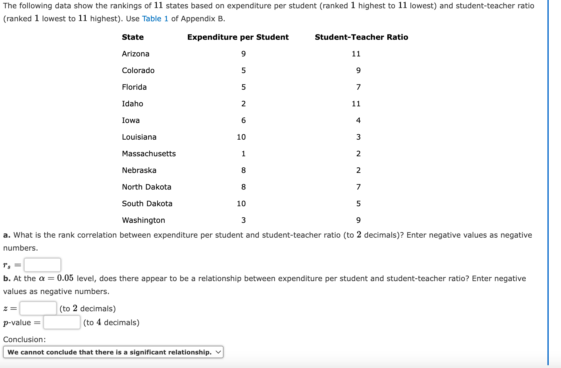
TABLE 1 CUMULATIVE PROBABILITIES FOR THE STANDARD NORMAL DISTRIBUTION Cumulative probability Entries in the table give the area under the curve to the left of the z value. For example, for z=-85, the cumulative probability is .1977. Z 0 Z .00 .01 .02 .03 .04 .05 .06 .07 .08 .09 -3.0 .0013 .0013 .0013 .0012 .0012 .0011 .0011 .0011 .0010 .0010 -2.9 .0019 .0018 .0018 .0017 .0016 .0016 .0015 .0015 .0014 .0014 -2.8 .0026 .0025 .0024 .0023 .0023 .0022 .0021 .0021 .0020 .0019 -2.7 .0035 .0034 .0033 .0032 .0031 .0030 .0029 .0028 .0027 .0026 -2.6 .0047 .0045 .0044 .0043 .0041 .0040 .0039 .0038 .0037 .0036 -2.5 .0062 .0060 .0059 .0057 .0055 .0054 .0052 .0051 .0049 .0048 -2.4 .0082 .0080 .0078 .0075 .0073 .0071 .0069 .0068 .0066 .0064 -2.3 .0107 .0104 .0102 .0099 .0096 .0094 .0091 .0089 .0087 .0084 -2.2 .0139 .0136 .0132 .0129 .0125 .0122 .0119 .0116 .0113 .0110 -2.1 .0179 .0174 .0170 .0166 .0162 .0158 .0154 .0150 .0146 .0143 -2.0 .0228 .0222 .0217 .0212 .0207 .0202 .0197 .0192 .0188 .0183 -1.9 .0287 .0281 .0274 .0268 .0262 .0256 .0250 .0244 .0239 .0233 -1.8 .0359 .0351 .0344 .0336 .0329 .0322 .0314 .0307 .0301 .0294 -1.7 .0446 .0436 .0427 .0418 .0409 .0401 .0392 .0384 .0375 .0367 -1.6 .0548 .0537 .0526 -1.5 .0668 .0655 .0643 .0630 .0516 .0505 .0618 .0495 .0485 .0475 .0465 .0455 .0606 .0594 .0582 .0571 .0559 1.4 .0808 .0793 .0778 .0764 .0749 .0735 .0721 .0708 .0694 .0681 -1.3 .0968 .0951 .0934 .0918 .0901 .0885 .0869 .0853 .0838 .0823 -1.2 .1151 .1131 .1112 .1093 .1075 .1056 .1038 .1020 .1003 .0985 -1.1 .1357 .1335 .1314 .1292 .1271 .1251 .1230 .1210 .1190 .1170 -1.0 .1587 .1562 .1539 .1515 .1492 .1469 .1446 .1423 .1401 .1379 -.9 .1841 .1814 .1788 .1762 .1736 .1711 .1685 .1660 .1635 .1611 -.8 .2119 .2090 .2061 .2033 .2005 .1977 .1949 .1922 .1894 .1867 -.7 .2420 2389 .2358 .2327 .2296 .2266 .2236 .2206 .2177 .2148 -.6 .2743 -.5 .3085 .2709 .2676 .3050 .2643 .2611 .2578 .2546 .2514 .2483 .2451 .3015 .2981 .2946 .2912 .2877 .2843 .2810 .2776 -.4 .3446 .3409 .3372 3336 .3300 .3264 3228 3192 .3156 3121 -3 .3821 .3783 .3745 .3707 .3669 .3632 .3594 .3557 .3520 .3483 -.2 .4207 .4168 .4129 4090 .4052 .4013 .3974 .3936 .3897 3859 -.1 .4602 .4562 .4522 .4483 4443 .4404 .4364 .4325 .4286 .4247 -.0 .5000 .4960 4920 .4880 .4840 .4801 .4761 .4721 .4681 .4641 Z Cumulative probability Entries in the table give the area under the curve to the left of the z value. For example, for z=1.25, the cumulative probability is .8944. Z .00 .01 .02 .03 .04 .05 .06 .07 .08 .09 .0 .5160 .1 .5000 .5040 .5080 .5120 .5398 .5438 .5478 .5517 .5557 .5596 .5636 .5675 .5714 .5753 .2 .5793 .5832 .5871 .5910 .5948 .5987 .6026 .6064 .6103 .6141 .3 .6179 .6217 .6255 .6293 .6331 .6368 .4 .6554 .6591 .6628 .6664 .6700 .6736 .5199 .5239 .5279 .5319 .5359 .6406 .6443 .6480 .6772 .6808 .6844 .6517 .6879 .5 .6 .6915 .6950 .7257 .7291 .7 .7580 .7611 .7642 .7673 .8 .7881 .7910 .7939 .7967 .9 .8159 .8186 .8212 .8238 .8264 9922 93 92223 2 1.0 .8413 .8438 .8461 .8485 .8508 1.1 .8643 .8665 .8686 .8708 .8729 1.2 .8849 .8869 .8888 .8907 .8925 1.3 .9032 .9049 .9066 .9082 1.4 .9192 .9207 .9222 .9236 .6985 .7019 .7054 .7088 .7324 .7357 .7389 .7422 .7704 .7734 .7764 .7794 .7823 .7995 .8023 .8051 .8078 .8106 .8289 .8315 .8340 .8531 .8554 .8577 .8749 .7123 .7157 .7190 .7224 .7454 .7486 .7517 .7549 .7852 .8133 .8365 .8389 .8599 .8621 .8944 .8770 .8790 .8962 .8980 .8997 .9015 .8810 .8830 .9099 .9115 .9251 .9265 .9131 .9147 .9162 .9177 .9279 .9292 .9306 .9319 1.5 1.6 .9332 .9345 .9357 .9370 .9452 .9463 .9474 .9484 .9382 .9394 .9495 .9505 .9406 .9418 .9429 .9441 .9515 .9525 .9535 .9545 2.6 .9901 .9904 .9925 .9927 .9940 .9941 .9943 .9945 .9953 .9955 .9956 .9957 .9959 2.7 .9965 .9966 .9967 .9968 .9969 2.8 .9974 .9975 .9976 .9977 .9977 .9981 .9982 .9982 .9983 .9984 .9984 .9987 .9987 .9987 .9988 .9988 .9989 3.0 .9693 .9699 .9706 1.9 2.0 2.1 2.2 2.3 .9713 .9719 .9726 .9772 .9778 .9783 .9788 .9793 .9821 .9826 .9830 .9834 .9838 .9861 .9864 .9868 .9871 .9875 .9893 .9896 .9898 2.4 .9918 .9920 .9922 2.5 .9938 .9732 .9738 .9744 .9750 .9756 .9761 .9767 .9798 .9803 .9808 .9812 .9817 .9842 .9846 .9850 .9854 .9857 .9878 .9881 .9884 .9887 .9890 .9906 .9909 .9911 .9913 .9916 .9929 .9931 .9932 .9934 .9936 .9946 .9948 .9949 .9951 .9960 .9961 .9962 .9963 .9952 .9964 .9970 .9971 .9972 .9973 .9974 .9978 .9979 .9979 .9980 .9981 .9985 .9985 .9986 .9989 .9990 .9990 .9986 .9989 1.7 .9554 .9564 .9573 .9582 .9591 .9599 .9608 .9616 .9625 .9633 1.8 .9641 .9649 .9656 .9664 .9671 .9678 .9686 The following data show the rankings of 11 states based on expenditure per student (ranked 1 highest to 11 lowest) and student-teacher ratio (ranked 1 lowest to 11 highest). Use Table 1 of Appendix B. State Arizona Colorado Expenditure per Student 9 Student-Teacher Ratio 11 6 5 Florida 5 7 Idaho 2 11 Iowa 6 4 Louisiana 10 Massachusetts 1 3 2 Nebraska 00 8 2 North Dakota 8 7 South Dakota Washington 10 3 5 9 a. What is the rank correlation between expenditure per student and student-teacher ratio (to 2 decimals)? Enter negative values as negative numbers. r s = b. At the = 0.05 level, does there appear to be a relationship between expenditure per student and student-teacher ratio? Enter negative values as negative numbers. x = p-value Conclusion: (to 2 decimals) (to 4 decimals) We cannot conclude that there is a significant relationship.
Step by Step Solution
There are 3 Steps involved in it
Step: 1

Get Instant Access to Expert-Tailored Solutions
See step-by-step solutions with expert insights and AI powered tools for academic success
Step: 2

Step: 3

Ace Your Homework with AI
Get the answers you need in no time with our AI-driven, step-by-step assistance
Get Started


