$\backslash$table$[[,$A$,$B$,$c$,$D$,$E$,$F$,$G$,$H$,,$J$,$K$,$L$,$M$,$N$,0,$p$],[1,$My Finances$],[2,,,,,,,,,,,,,,,,],[3,],[4,$Income,$$0\mathrm{.}00,$$$0\mathrm{.}00,$$$0\mathrm{.}00,$$$0\mathrm{.}00,$$$0\mathrm{.}00,$$$100\mathrm{.}00,$$$150\mathrm{.}00,$$$0\mathrm{.}00,$$$0\mathrm{.}00,$$$0\mathrm{.}00,$$$0\mathrm{.}00,$$$0\mathrm{.}00,$$$250\mathrm{.}00,$$$20\mathrm{.}83,],[5,$Clothing,$$0\mathrm{.}00,$$$0\mathrm{.}00,$$$0\mathrm{.}00,$$$0\mathrm{.}00,$$$0\mathrm{.}00,$$$0\mathrm{.}00,$$$0\mathrm{.}00,$$$0\mathrm{.}00,$$$0\mathrm{.}00,$$$0\mathrm{.}00,$$$0\mathrm{.}00,$$$0\mathrm{.}00,$$$0\mathrm{.}00,$$$0\mathrm{.}00,],[6,$Entertainment,$$0\mathrm{.}00,$$$0\mathrm{.}00,$$$0\mathrm{.}00,$$$0\mathrm{.}00,$$$0\mathrm{.}00,$$$0\mathrm{.}00,$$$0\mathrm{.}00,$$$0\mathrm{.}00,$$$0\mathrm{.}00,$$$0\mathrm{.}00,$$$0\mathrm{.}00,$$$0\mathrm{.}00,$$$0\mathrm{.}00,$$$0\mathrm{.}00,],[7,$Groceries,$$0\mathrm{.}00,$$$30\mathrm{.}00,($$$40\mathrm{.}00),$$$10\mathrm{.}00,$$$0\mathrm{.}00,$$$0\mathrm{.}00,($$$50\mathrm{.}00),$$$0\mathrm{.}00,$$$15\mathrm{.}00,$$$0\mathrm{.}00,$$$0\mathrm{.}00,$$$0\mathrm{.}00,($$$35\mathrm{.}00),($$$2\mathrm{.}92),],[8,$Insurance,$$0\mathrm{.}00,$$$0\mathrm{.}00,$$$0\mathrm{.}00,$$$0\mathrm{.}00,$$$0\mathrm{.}00,$$$0\mathrm{.}00,$$$0\mathrm{.}00,$$$0\mathrm{.}00,$$$0\mathrm{.}00,$$$0\mathrm{.}00,$$$0\mathrm{.}00,$$$0\mathrm{.}00,$$$0\mathrm{.}00,$$$0\mathrm{.}00,],[9,$Rent,$$0\mathrm{.}00,$$$0\mathrm{.}00,$$$0\mathrm{.}00,$$$0\mathrm{.}00,$$$0\mathrm{.}00,$$$0\mathrm{.}00,$$$50\mathrm{.}00,$$$50\mathrm{.}00,$$$50\mathrm{.}00,$$$50\mathrm{.}00,$$$50\mathrm{.}00,$$$50\mathrm{.}00,$$$300\mathrm{.}00,$$$25\mathrm{.}00,],[10,$Transportation,$$0\mathrm{.}00,$$$0\mathrm{.}00,$$$0\mathrm{.}00,$$$0\mathrm{.}00,$$$0\mathrm{.}00,$$$0\mathrm{.}00,$$$0\mathrm{.}00,$$$0\mathrm{.}00,$$$0\mathrm{.}00,$$$0\mathrm{.}00,$$$0\mathrm{.}00,$$$0\mathrm{.}00,$$$0\mathrm{.}00,$$$0\mathrm{.}00,],[11,$Utilities,$$25\mathrm{.}00,$$$25\mathrm{.}00,$$$25\mathrm{.}00,$$$25\mathrm{.}00,$$$0\mathrm{.}00,($$$10\mathrm{.}00),($$$20\mathrm{.}00),($$$10\mathrm{.}00),$$$0\mathrm{.}00,($$$25\mathrm{.}00),($$$25\mathrm{.}00),$$$0\mathrm{.}00,$$$10\mathrm{.}00,$$$0\mathrm{.}83,],[12,$Misc.,$$50\mathrm{.}00,$$$0\mathrm{.}00,$$$25\mathrm{.}00,$$$50\mathrm{.}00,$$$0\mathrm{.}00,$$$0\mathrm{.}00,$$$10\mathrm{.}00,$$$0\mathrm{.}00,($$$15\mathrm{.}00),$$$0\mathrm{.}00,$$$0\mathrm{.}00,$$$180\mathrm{.}00,$$$300\mathrm{.}00,$$$25\mathrm{.}00,],[13,$Savings Deposit,$($$$75\mathrm{.}00),($$$55\mathrm{.}00),($$$10\mathrm{.}00),($$$85\mathrm{.}00),$$$0\mathrm{.}00,$$$110\mathrm{.}00,$$$160\mathrm{.}00,($$$40\mathrm{.}00),($$$50\mathrm{.}00),($$$25\mathrm{.}00),($$$25\mathrm{.}00),($$$230\mathrm{.}00),($$$325\mathrm{.}00),($$$27\mathrm{.}08),],[14],[15,$Savings Balance,$($$$75\mathrm{.}00),($$$130\mathrm{.}00),($$$140\mathrm{.}00),($$$225\mathrm{.}00),($$$225\mathrm{.}00),\backslash$table$[[($$$115\mathrm{.}00)]],$$$45\mathrm{.}00,$$$5\mathrm{.}00,($$$45\mathrm{.}00),($$$70\mathrm{.}00),($$$95\mathrm{.}00),($$$325\mathrm{.}00),,,],[16],[18],[19],[20],[21],[22],[23],[24],[25],[,>,,$D$\_,$ferences,$+,,,,,$vdots,E$,=,,=,,]]$please answer this question in detialed steps for a beginner

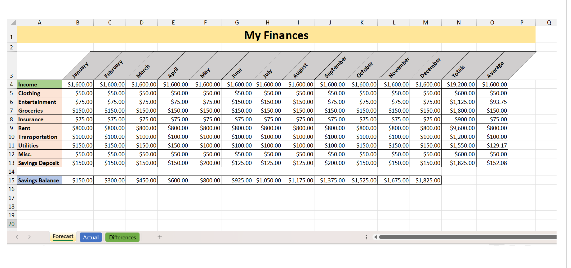
Your project will be to recreate the Excel workbook shown at the bottom of this document. The workbook will contain three worksheets named $$Forecast$,$Actual$$ and $$Differences$.$ The worksheet tabs should be colored as shown.

First, create the $$Forecast$$ worksheet, exactly as shown below, paying particular attention to the following:

Create a Custom Header with the FileName field in the left section, and the Date field in the right section.

The title $($My Finances$)$ is merged and centered in row $1,$ across columns A through P$.$

The columns headings $$January$$ through $$Average$$ are slanted $45$ degrees.

The row headings $$Income$$ through $$Savings Balance$$ are shaded in different hues.

The cells containing the monthly data for Income, Clothing, Entertainment, Groceries, Insurance, Rent, Transportation, Utilities and Other must be keyed into the corresponding cells.

The cells containing the data for Savings Deposit, Savings Balance, Total and Average are all calculated fields, populated using equations or functions. The data in these cells must NOT be keyed in directly.

All of the numeric fields must be formatted exactly as shown.

When you have completed the $$Forecast$$ worksheet, copy it into a new worksheet named $$Actual$.$ Modify this worksheet exactly as shown below, paying particular attention to the following:

Some of the dollar amounts in the cells will need to be changed $($to match the image below$).$ This reflects the real world reality that a budget is an estimate, and sometimes things don$$t go exactly as we originally expected.

If you set up the calculated fields correctly in the original $$Forecast$$ worksheet, they will continue to yield the correct result in this $$Actual$$ worksheet, after you make the necessary changes to the monthly data.

You must insert a column chart $($as shown in the image below$),$ which shows the amount of the $$Savings Deposit$,$ by month.

When you have completed the $$Actual$$ worksheet, make another copy of the $$Forecast$$ worksheet into a new worksheet named $$Differences$.$ Modify this worksheet exactly as shown below, paying particular attention to the following:

All of the numeric fields on this worksheet are the result of subtracting the value in the corresponding cell in the $$Forecast$$ worksheet from the value in the corresponding cell in the $$Actual$$ worksheet $($Actual minus Forecast$).$ These are all calculated fields and must NOT be keyed in directly.

Using Conditional Formatting, highlight only those cells in the worksheet which contain a value other than zero. You may use any highlighting color that you wish.

When you have successfully completed all three worksheets in the workbook, save the workbook as $$ExcelFinal$-$YourName$$ and submit.