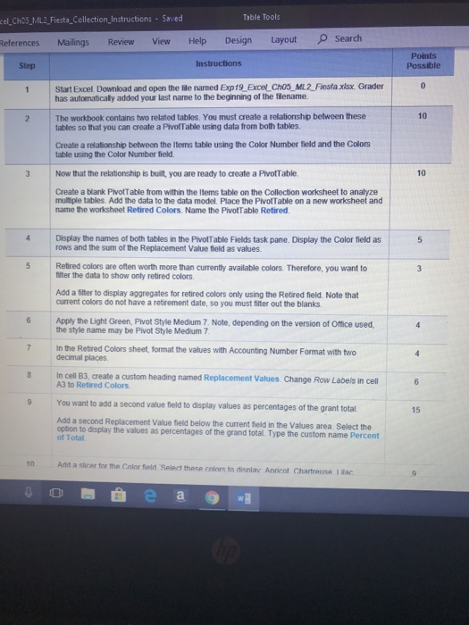
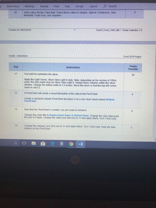
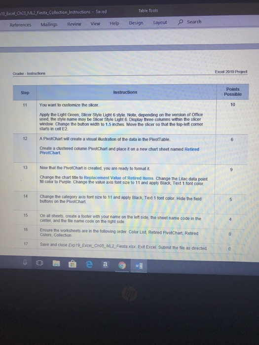
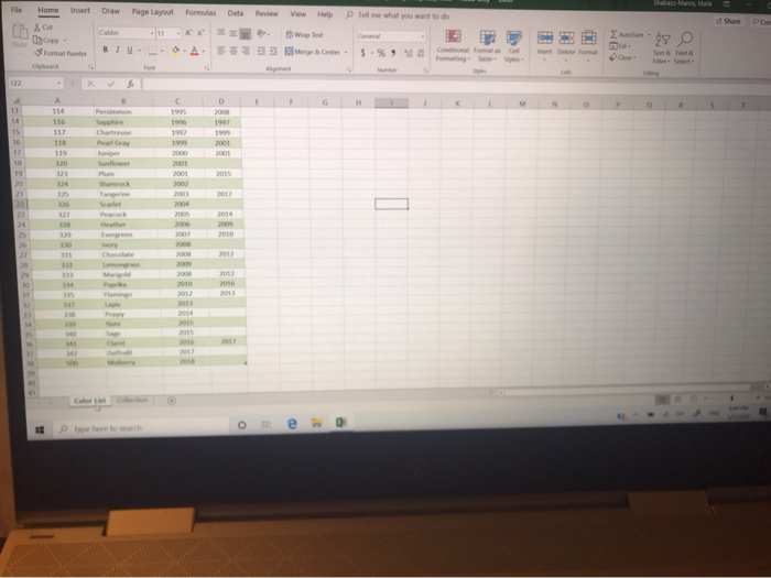
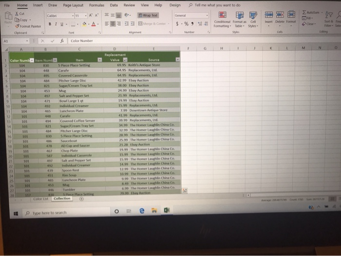
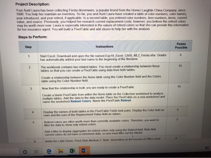
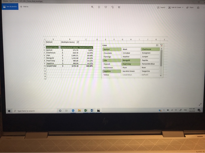
Table Tools cel_CHOS_ML2_Fiesta Collection Instructions - Saved References Mailings Review View Help Design Layout Search Points Possible Step Instructions Start Excel. Download and open the file narned Exp19_Excel Cho5_ML2_Fiesta.xlsx. Grader has automatically added your last name to the beginning of the filename. The workbook contains two related tables. You must create a relationship between these tables so that you can create a Pivot Table using data from both tables Create a relationship between the items table using the Color Number field and the Colors table using the Color Number field. Now that the relationship is built, you are ready to create a Pivottable. Create a blank Pivot Table from within the Items table on the Collection worksheet to analyze multiple tables. Add the data to the data model. Place the Pivo Table on a new worksheet and name the worksheet Retired Colors. Name the Pivot Table Retired. Display the names of both tables in the PivotTable Fields task pane. Display the Color field as rows and the sum of the Replacement Value field as values Retired colors are often worth more than currently available colors. Therefore, you want to filter the data to show only retired colors Add a filter to display aggregates for retired colors only using the Retired field. Note that current colors do not have a retirement date, so you must filter out the blanks Apply the Light Green, Pivot Style Medium 7. Note, depending on the version of Office used, the style name may be Pivot Style Medium 7. In the Retired Colors sheet, format the values with Accounting Number Format with two decimal places In cell B3, create a custom heading named Replacement Values. Change Row Labels in cell A3 to Retired Colors 9 You want to add a second value field to display values as percentages of the grant total. Add a second Replacement Value field below the current field in the values area Select the option to display the values as percentages of the grand total Type the custom name Percent of Total 10 Add a slicer for the Color field Select these colors to dislav Anrient Chartreuse llac References 10 Mailings Review View Help Design Layout Search Add a slicer for the Color field. Select these colors to display Apricot Chartreuse, Lilac Marigold Pearl Grey, and Sapphire. Created On: 05222019 bip19 L el ChOS ML2 - Fiesta Collection 10 Grader - Instruction Excel 2019 Prod Step Points Instructions Possible You want to customize the slicer Apply the Light Green, Slicer Style Light 6 style Note depending on the version of Office used, the style name may be Slicer Style Light 6 Display three columns within the sicer window Change the button width to 1.5 inches. Move the slicer so that the top left corner starts in cell E2 A PivotChart will create a visual illustration of the data in the Pivot Table Create a clustered column PivotChart and place it on a new chart sheet named Retired PivotChart Now that the PivotChart is created, you are ready to format it Change the chart title to Replacement Value of Retired Items Change the data point il color to Purple Change the value as font size to 11 and apply Black Text 1 font color Change the category as font size to 11 and apply Black Text 1 font color. Hide the field buttons on the PivotChart. JO e a wg Table Tools 19_Excel Cho5_ML2 Fiesta_Collection Instructions. Saved References Mailings Review View Help Design Layout Search Grader-Instructions Excel 2019 Project Step Instructions Points Possible You want to customize the slicer Apply the Light Green Slicer Style Light 6 style Note depending on the version of Office used, the style name may be Slicer Style Light 6. Display three columns within the slicer window. Change the button width to 1.5 inches. Move the slicer so that the top-left corner starts in cell E2 A PivotChart will create a visual illustration of the data in the PivotTable Create a clustered column PivotChart and place it on a new chart sheet named Retired PivotChart Now that the PivotChart is created, you are ready to format it Change the chart title to Replacement Value of Retired Items Change the Lilac data point fill color to Purple Change the value as font size to 11 and apply Black Text 1 font color Change the category axis font size to 11 and apply Black, Text 1 font color. Hide the field buttons on the PivotChart. On all sheets, create a footer with your name on the left side, the sheet name code in the center, and the file name code on the right side Ensure the worksheets are in the following order Color List, Retired PivotChart Retired Colors Collection 17 Save and close Exp19_Excel_CHO_ML2_Fiestaxlsx Exit Excel Submit the file as directed DOB e a wg File Insert Draw Page Layout Formulas Data Review View Help Time what you want to do Share PC Home - 20 P etere to watch LOWO File Home Insert Draw Data Review Page Layout 11 O Formulas AA . A Caliburi BIV View Help Design Wrap Text Center - $ .% EE Entus- Copy from Tell me what you want to do EE . Condtional Format as Cell Formatting table Styles Styles Insert Delete Format inter Chyboard X Color Number Color Numm um 830 er Spiece Place Setting Covered Casserole Pitcher Large Disc eray Set 104 S 104 Replacement Value 6.95 Keith's Antique Store A la Replac e d Thayetion O by Auction 24 thay Action 21.99 Replacements, the 1999 by Auction 15. Replacements, 7.99 Downtown Antique Store 41.99 Replacements, 19. Replacements, Lid 1.9 The Home Laughlin China Co. 32. The Home Layhin China Co. 2.99 The Home Lwin China Coc 25.99 The Home in China Co. 21.28 bay Auction 19.09 The Home Cina Coc 159 The Home Cina C 15 The Home Cinco Salt and pepper Set Bowl Large 1 Individual Creamer Luncheon Plate Carate Covered Coffee Server Sugar Cream Tray Set Patcher Large Disc 5 Pece Plate Setting 101 AD Cup and Saucer Chop Plate Oy Salt and pepper Set 101 101 Soon Rest 12 The Chica 10 The 101 6 The Home Cina C Piece Pace Setting Collection Color List Type here to search o e o Project Description: Your Aunt Laura has been collecting Fiesta dinnerware, a popular brand from the Homer Laughlin China Company, since 1986. You help her maintain an inventory So far, you and Aunt Laura have created a table of color numbers, color names year introduced, and year retired, if applicable. In a second table, you entered color numbers, item numbers, items, current value, and source. Previously, you helped her research current replacement costs, however, you believe the retired colors may be worth more now. Laura is especially interested in the values of retired colors so that she can provide this information for her insurance agent. You will build a Pivot Table and add slicers to help her with the analysis Steps to Perform: Step Instructions Points Possible Start Excel Download and open the file named Exp19 Excel Ch05 ML2 Fiesta xlsx Grader has automatically added your last name to the beginning of the filename. The workbook contains two related tables. You must create a relationship between these tables so that you can create a Pivot Table using data from both tables Create a relationship between the items table using the Color Number field and the Colors table using the Color Number field. Now that the relationship is built, you are ready to create a Pivot Table Create a blank Pivot Table from within the items table on the Collection worksheet to analyze multiple tables. Add the data to the data model. Place the Pivot Table on a new worksheet and name the worksheet Retired Colors Name the Pivot Table Retired Display the names of both tables in the Pivot Table Fields task pane Display the Color Geld as rows and the sum of the Replacement Value field as values Retired colors are often worth more than currently available colors. Therefore, you want to filter the data to show only retired colors Add a filter to display aggregates for retired colors only using the Retired field Note that current colors do not have a retirement date, so you must hiter out the blanks o men Anthelinten Privative Medium 7 Note denne on the w + Such tatt Share U Retired Colors aparentes Percent of Total 5 Chartreuse 640 2335 MON Choco Evergreen 7 Marigold 10.11 Marigold Pearl Gray Perwiele Sea Mist Green Cobalt Type here to search Table Tools cel_CHOS_ML2_Fiesta Collection Instructions - Saved References Mailings Review View Help Design Layout Search Points Possible Step Instructions Start Excel. Download and open the file narned Exp19_Excel Cho5_ML2_Fiesta.xlsx. Grader has automatically added your last name to the beginning of the filename. The workbook contains two related tables. You must create a relationship between these tables so that you can create a Pivot Table using data from both tables Create a relationship between the items table using the Color Number field and the Colors table using the Color Number field. Now that the relationship is built, you are ready to create a Pivottable. Create a blank Pivot Table from within the Items table on the Collection worksheet to analyze multiple tables. Add the data to the data model. Place the Pivo Table on a new worksheet and name the worksheet Retired Colors. Name the Pivot Table Retired. Display the names of both tables in the PivotTable Fields task pane. Display the Color field as rows and the sum of the Replacement Value field as values Retired colors are often worth more than currently available colors. Therefore, you want to filter the data to show only retired colors Add a filter to display aggregates for retired colors only using the Retired field. Note that current colors do not have a retirement date, so you must filter out the blanks Apply the Light Green, Pivot Style Medium 7. Note, depending on the version of Office used, the style name may be Pivot Style Medium 7. In the Retired Colors sheet, format the values with Accounting Number Format with two decimal places In cell B3, create a custom heading named Replacement Values. Change Row Labels in cell A3 to Retired Colors 9 You want to add a second value field to display values as percentages of the grant total. Add a second Replacement Value field below the current field in the values area Select the option to display the values as percentages of the grand total Type the custom name Percent of Total 10 Add a slicer for the Color field Select these colors to dislav Anrient Chartreuse llac References 10 Mailings Review View Help Design Layout Search Add a slicer for the Color field. Select these colors to display Apricot Chartreuse, Lilac Marigold Pearl Grey, and Sapphire. Created On: 05222019 bip19 L el ChOS ML2 - Fiesta Collection 10 Grader - Instruction Excel 2019 Prod Step Points Instructions Possible You want to customize the slicer Apply the Light Green, Slicer Style Light 6 style Note depending on the version of Office used, the style name may be Slicer Style Light 6 Display three columns within the sicer window Change the button width to 1.5 inches. Move the slicer so that the top left corner starts in cell E2 A PivotChart will create a visual illustration of the data in the Pivot Table Create a clustered column PivotChart and place it on a new chart sheet named Retired PivotChart Now that the PivotChart is created, you are ready to format it Change the chart title to Replacement Value of Retired Items Change the data point il color to Purple Change the value as font size to 11 and apply Black Text 1 font color Change the category as font size to 11 and apply Black Text 1 font color. Hide the field buttons on the PivotChart. JO e a wg Table Tools 19_Excel Cho5_ML2 Fiesta_Collection Instructions. Saved References Mailings Review View Help Design Layout Search Grader-Instructions Excel 2019 Project Step Instructions Points Possible You want to customize the slicer Apply the Light Green Slicer Style Light 6 style Note depending on the version of Office used, the style name may be Slicer Style Light 6. Display three columns within the slicer window. Change the button width to 1.5 inches. Move the slicer so that the top-left corner starts in cell E2 A PivotChart will create a visual illustration of the data in the PivotTable Create a clustered column PivotChart and place it on a new chart sheet named Retired PivotChart Now that the PivotChart is created, you are ready to format it Change the chart title to Replacement Value of Retired Items Change the Lilac data point fill color to Purple Change the value as font size to 11 and apply Black Text 1 font color Change the category axis font size to 11 and apply Black, Text 1 font color. Hide the field buttons on the PivotChart. On all sheets, create a footer with your name on the left side, the sheet name code in the center, and the file name code on the right side Ensure the worksheets are in the following order Color List, Retired PivotChart Retired Colors Collection 17 Save and close Exp19_Excel_CHO_ML2_Fiestaxlsx Exit Excel Submit the file as directed DOB e a wg File Insert Draw Page Layout Formulas Data Review View Help Time what you want to do Share PC Home - 20 P etere to watch LOWO File Home Insert Draw Data Review Page Layout 11 O Formulas AA . A Caliburi BIV View Help Design Wrap Text Center - $ .% EE Entus- Copy from Tell me what you want to do EE . Condtional Format as Cell Formatting table Styles Styles Insert Delete Format inter Chyboard X Color Number Color Numm um 830 er Spiece Place Setting Covered Casserole Pitcher Large Disc eray Set 104 S 104 Replacement Value 6.95 Keith's Antique Store A la Replac e d Thayetion O by Auction 24 thay Action 21.99 Replacements, the 1999 by Auction 15. Replacements, 7.99 Downtown Antique Store 41.99 Replacements, 19. Replacements, Lid 1.9 The Home Laughlin China Co. 32. The Home Layhin China Co. 2.99 The Home Lwin China Coc 25.99 The Home in China Co. 21.28 bay Auction 19.09 The Home Cina Coc 159 The Home Cina C 15 The Home Cinco Salt and pepper Set Bowl Large 1 Individual Creamer Luncheon Plate Carate Covered Coffee Server Sugar Cream Tray Set Patcher Large Disc 5 Pece Plate Setting 101 AD Cup and Saucer Chop Plate Oy Salt and pepper Set 101 101 Soon Rest 12 The Chica 10 The 101 6 The Home Cina C Piece Pace Setting Collection Color List Type here to search o e o Project Description: Your Aunt Laura has been collecting Fiesta dinnerware, a popular brand from the Homer Laughlin China Company, since 1986. You help her maintain an inventory So far, you and Aunt Laura have created a table of color numbers, color names year introduced, and year retired, if applicable. In a second table, you entered color numbers, item numbers, items, current value, and source. Previously, you helped her research current replacement costs, however, you believe the retired colors may be worth more now. Laura is especially interested in the values of retired colors so that she can provide this information for her insurance agent. You will build a Pivot Table and add slicers to help her with the analysis Steps to Perform: Step Instructions Points Possible Start Excel Download and open the file named Exp19 Excel Ch05 ML2 Fiesta xlsx Grader has automatically added your last name to the beginning of the filename. The workbook contains two related tables. You must create a relationship between these tables so that you can create a Pivot Table using data from both tables Create a relationship between the items table using the Color Number field and the Colors table using the Color Number field. Now that the relationship is built, you are ready to create a Pivot Table Create a blank Pivot Table from within the items table on the Collection worksheet to analyze multiple tables. Add the data to the data model. Place the Pivot Table on a new worksheet and name the worksheet Retired Colors Name the Pivot Table Retired Display the names of both tables in the Pivot Table Fields task pane Display the Color Geld as rows and the sum of the Replacement Value field as values Retired colors are often worth more than currently available colors. Therefore, you want to filter the data to show only retired colors Add a filter to display aggregates for retired colors only using the Retired field Note that current colors do not have a retirement date, so you must hiter out the blanks o men Anthelinten Privative Medium 7 Note denne on the w + Such tatt Share U Retired Colors aparentes Percent of Total 5 Chartreuse 640 2335 MON Choco Evergreen 7 Marigold 10.11 Marigold Pearl Gray Perwiele Sea Mist Green Cobalt Type here to search
