Thanks a lot!!!
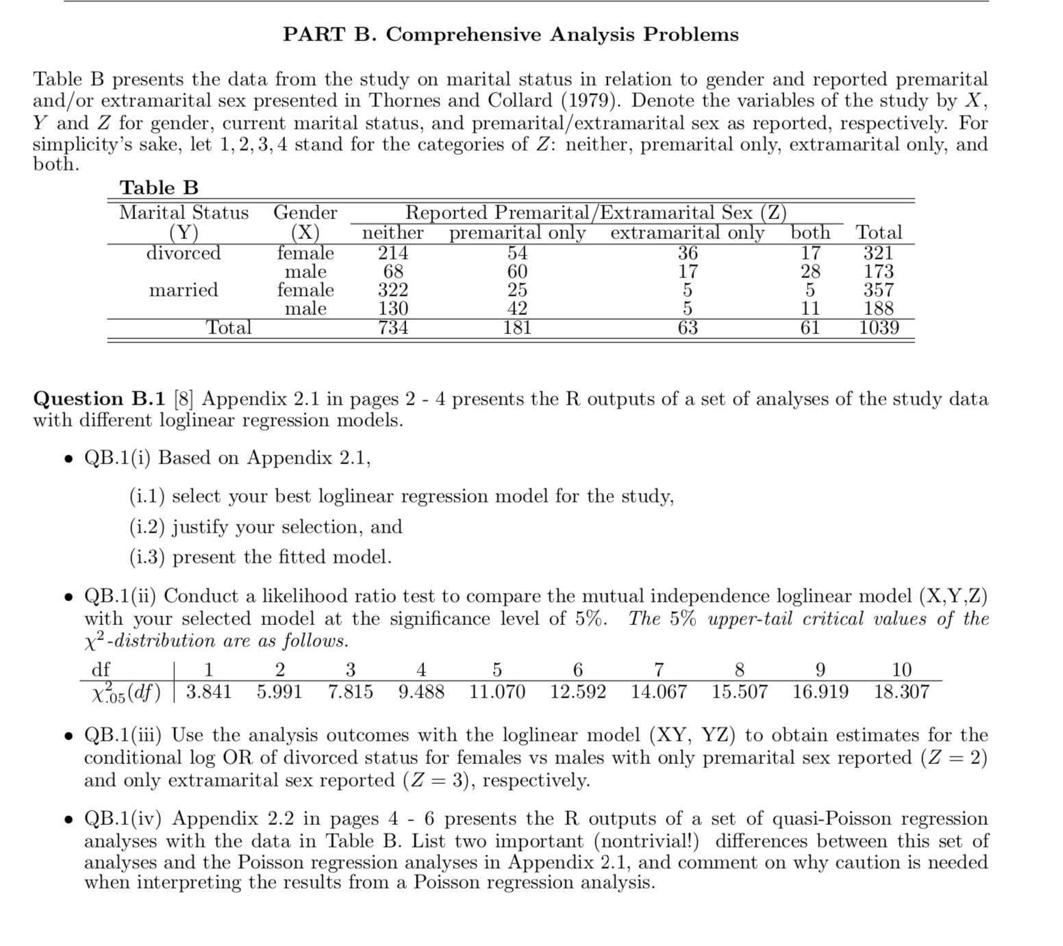
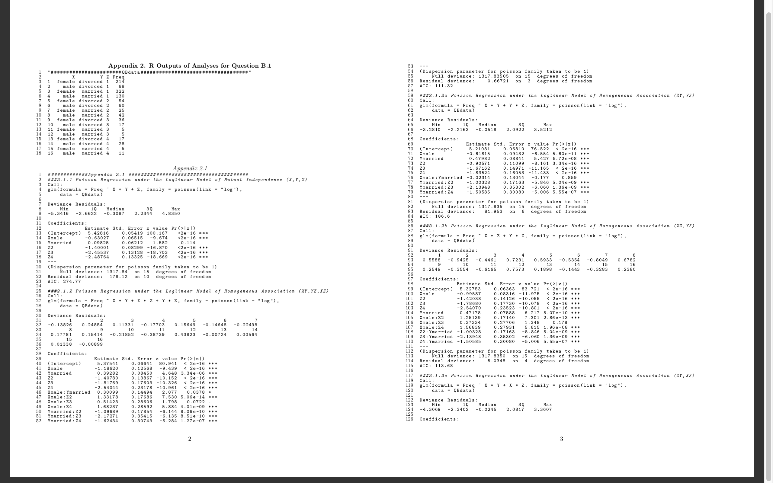
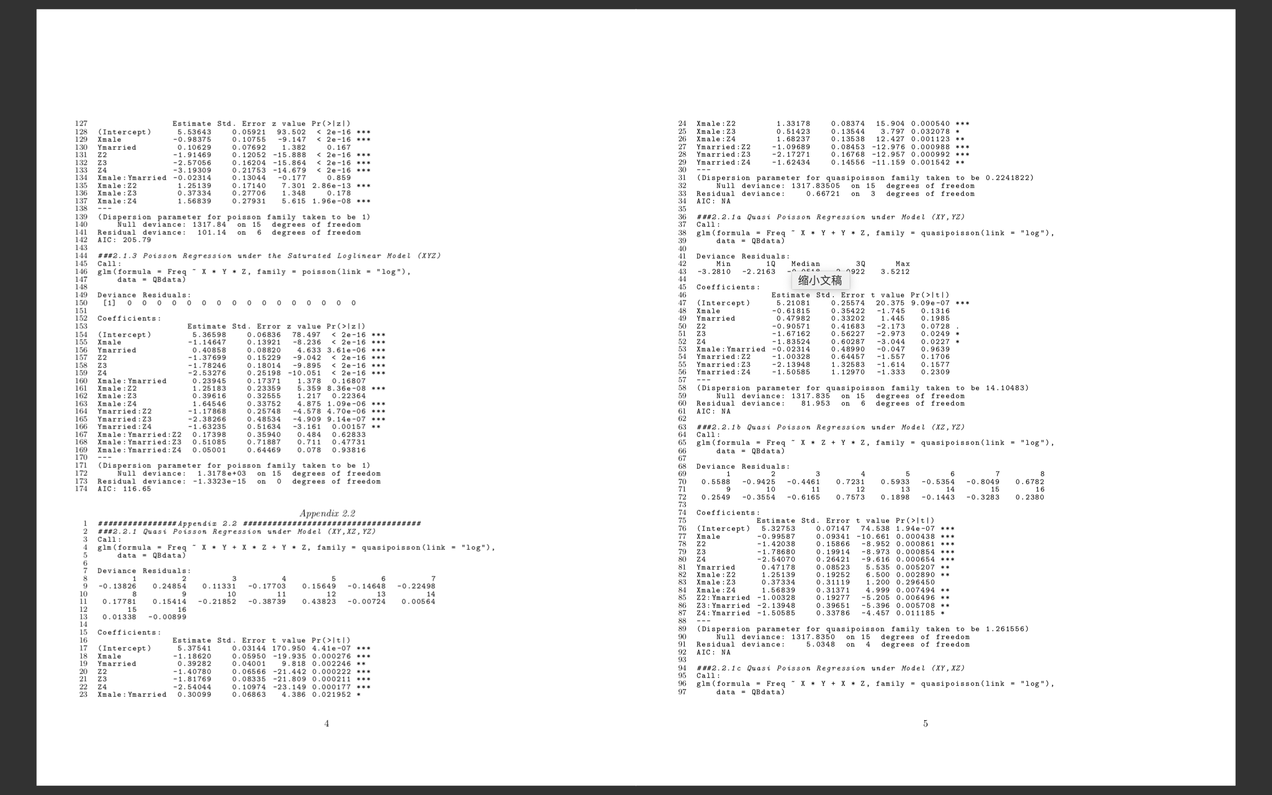
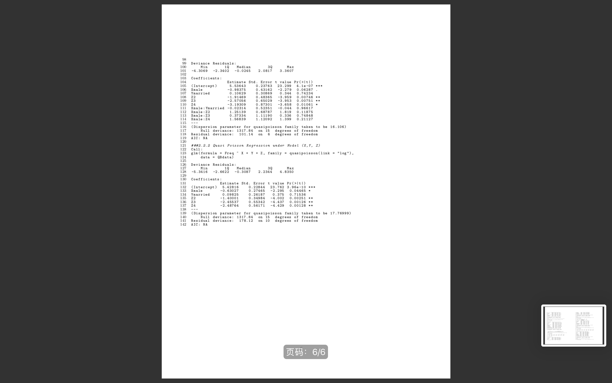
PART B. Comprehensive Analysis Problems Table B presents the data from the study on marital status in relation to gender and reported premarital and/or extramarital sex presented in Thornes and Collard (1979). Denote the variables of the study by X, Y and Z for gender, current marital status, and premarital/ extramarital sex as reported, respectively. For simplicity's sake, let 1, 2, 3, 4 stand for the categories of Z: neither, premarital only, extramarital only, and both. Table B Marital Status Gender Reported Premarital /Extramarital Sex (Z) ( Y) (X) neither premarital only extramarital only both Total divorced female 214 54 36 17 321 male 68 60 28 173 married female 322 25 5 357 male 130 42 11 188 Total 734 181 61 1039 Question B.1 [8] Appendix 2.1 in pages 2 - 4 presents the R outputs of a set of analyses of the study data with different loglinear regression models. . QB.1(i) Based on Appendix 2.1, (i.1) select your best loglinear regression model for the study, (i.2) justify your selection, and (i.3) present the fitted model. . QB.1(ii) Conduct a likelihood ratio test to compare the mutual independence loglinear model (X, Y,Z) with your selected model at the significance level of 5%. The 5% upper-tail critical values of the x2 -distribution are as follows. df 2 3 5 6 7 8 9 10 X.05 (df) |3.841 5.991 7.815 9.488 11.070 12.592 14.067 15.507 16.919 18.307 . QB.1(iii) Use the analysis outcomes with the loglinear model (XY, YZ) to obtain estimates for the conditional log OR of divorced status for females vs males with only premarital sex reported (Z = 2) and only extramarital sex reported (Z = 3), respectively. . QB.1(iv) Appendix 2.2 in pages 4 - 6 presents the R outputs of a set of quasi-Poisson regression analyses with the data in Table B. List two important (nontrivial!) differences between this set of analyses and the Poisson regression analyses in Appendix 2.1, and comment on why caution is needed when interpreting the results from a Poisson regression analysis.Appendix 2. R Outputs of Analyses for Question B.1 "# ##### ###### ###### #####QBdata###################################" (Dispersion parameter for poisson family taken to be 1) fema ivorced 214 1317 . 83505 on 15 degrees of freedom divorce 2 68 viance : 0 . 66721 on 3 degrees of freedom marr NNNNNN# AIC: 111 .32 fema W N a marrie emale divorced 54 Call : # ##2. 1. 2a Poisson Regression under the Loglinear Model of Homogeneous Association (XY, YZ) male divorced 2 60 married glm (formula = Freq emale 25 data = QBdataj X * Y + Y * Z, family = poisson (link = "log"), emale divorced 36 ale d female married 3 17 Deviance Residuals : Min 10 Median Max male married 3 . 2810 -2. 2163 -0. 0518 2. 0922 3. 5212 emale divor 17 nale 28 Coefficients : female Estimate Std. . Error z value Pr (> Izl) male married (Intercept) 5 . 21081 0 . 06810 76 .522 -0 . 61815 0 . 09432 |z1 ) ###2. 1. 2b Poisson Regression under the Loglinear Model of Homogeneous Association (XZ, YZ) (Intercept ) 5. 42816 0. 05419 100. 167 |z1 ) # ##2. 1.2 Poisson Regression under the Loglinear Model of Homogeneous Association (XY, YZ, XZ) (Intercept) 5. 32753 0. 06363 Call: Amale -0 . 99587 83 . 721 Itl) (Intercept ) 5 . 21081 0. 25574 20 .375 9. 09e-07 * * * Coefficients : Xmale -0 . 61815 0 35422 -1.745 Ymarried 1: 445 0. 1316 Estimate Std . Error 0 . 47982 0 . 33202 0. 1985 (Intercept ) value Pr (>|z) 42 0. 90571 5 . 36598 0 . 41683 -2. 173 0. 0728 Amale 1 . 14647 0 . 06836 78 . 497 -8.236 It!) (Intercept) 5. 53643 0 . 23763 23 . 299 4. 1e-07 .98375 0. 43162 -2.279 107 Xmale 0. 06287 Ymarried 0 . 10629 72 0 . 30869 0. 344 0.74234 1. 91469 109 -3.959 . 00746 -2. 57056 0 . 65029 -3.953 0. 00751 -3. 19309 0. 87301 -3.658 0. 01061 Xmale : Ymarried -0. 02314 0 . 52351 -0. 044 1 . 25139 0. 68787 1: 819 0.96617 0 11 875 Xmale : 23 0 . 37334 1. 11190 0. 74848 Xmale : Z4 1 . 56839 0 . 336 1 . 12092 1 . 399 0 . 21127 (Dispersion parameter for quasipoisson family taken to be 16. 106) Null deviance: 1317 .84 degrees of freedom Residual deviance: 101 . 14 on 15 IC : NA degrees of freedom Call : # ##2. 2.2 Quasi Poisson Regression under Model (X, Y, Z) glm (formula = Freq - X + Y + Z, family = quasipoisson(link = "log"), data = QBdata) Deviance Residuals: Min -2. 6622 Median Max -5 . 3416 -0. 3087 2. 2344 4 . 8350 130 Coefficients : 131 Estimate Std. Error t value Pr (>Itl ) 133 (Intercept) 5.42816 Xmale 0 . 22844 134 0. 63027 0 . 27465 -2.295 e -10 * * 4465 * married 0. 09825 0 . 26187 0. 375 0. 71536 Z2 -1. 40001 137 Z3 -2: 45537 0 . 34984 0 . 55342 -4.002 0. 00251 0 00126 * 74 -2. 48764 0 . 56171 -4.429 0. 00128 * * 138 139 (Dispersion parameter for quasipoisson family taken to be 17. 76999) 140 Null deviance: 1317 .84 on 15 degrees of freedom 142 Residual deviance: 178. 12 on 10 degrees of freedom AIC : NA DA Gy : 6/6


