 the book name Basic concepts computational physics
help plase

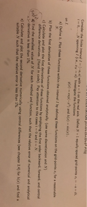
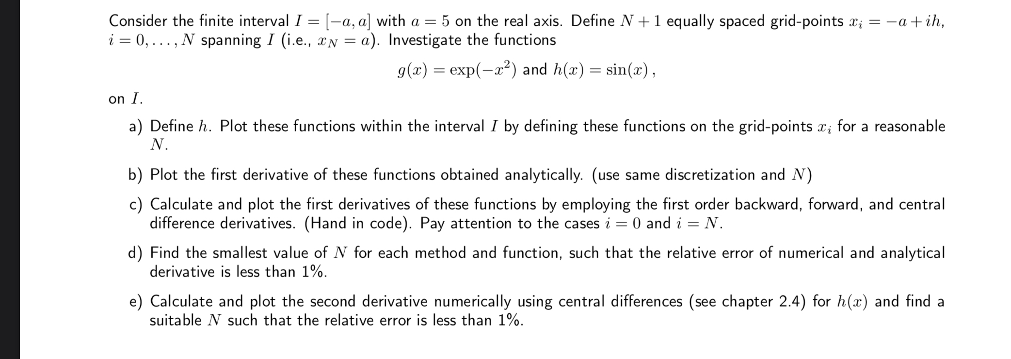
Consider the finite interval I = (-a, a) with a = 5 on the real axis. Define N +1 equally spaced grid-points Xi = -a +ih, i = 0, ..., N spanning I (i.e., XN = a). Investigate the functions g(x) = exp(-x2) and h(x) = sin(x), on I. a) Define h. Plot these functions within the interval I by defining these functions on the grid-points xi for a reasonable N. b) Plot the first derivative of these functions obtained analytically. (use same discretization and N) c) Calculate and plot the first derivatives of these functions by employing the first order backward, forward, and central difference derivatives. (Hand in code). Pay attention to the cases i = 0 and i = N. d) Find the smallest value of N for each method and function, such that the relative error of numerical and analytical derivative is less than 1%. e) Calculate and plot the second derivative numerically using central differences (see chapter 2.4) for h(x) and find a suitable N such that the relative error is less than 1%. Consider the finite interval/ -, al with a -5 on the real axis. Define N+1 equally spaced grid points 14 - ih i=0,..., N spanning I (ie, IN a). Investigate the functions 9(+) - exp(-x) and (3) - sin(), on 1. a) Define h. Plot these functions within the interval / by defining these functions on the grid points for a reasonable N b) Plot the first derivative of these functions obtained analytically. (use same discretization and N) c) Calculate and plot the first derivatives of these functions by employing the first order backward, forward, and central difference derivatives. (Hand in code). Pay attention to the cases i = 0 and i N . d) Find the smallest value of N for each method and function, such that the relative error of numerical and analytical derivative is less than 1%. e) Calculate and plot the second derivative numerically using central differences (sce chapter 2.4) for h(s) and find a suitable N such that the relative error is less than 1%. TIATION P+10+15+10+5* PTS) Consider the finite interval T -a, a) with a 5 on the real axis. Define N + 1 equally spaced grid-points . 1 0,..., spanning I (ie, IN = a). Investigate the functions g(x) = exp(-x) and (x) = sin(x), -atih on I. a) Define h. Plot these functions within the interval by defining these functions on the grid-points T, for a reasonable N. C b) Plot the first derivative of these functions obtained analytically. (use same discretization and N) c) Calculate and plot the first derivatives of these functions by employing the first order backward, forward, and central difference derivatives. (Hand in code). Pay attention to the cases i = 0 and i = N. .) Find the smallest value of N for each method and function, such that the relative error of numerical and analytical derivative is less than 1%. e) Calculate and plot the second derivative numerically using central differences (see chapter 2.4) for h() and find a suitable N such that the relative error is less than 1%. Consider the finite interval I = (-a, a) with a = 5 on the real axis. Define N +1 equally spaced grid-points Xi = -a +ih, i = 0, ..., N spanning I (i.e., XN = a). Investigate the functions g(x) = exp(-x2) and h(x) = sin(x), on I. a) Define h. Plot these functions within the interval I by defining these functions on the grid-points xi for a reasonable N. b) Plot the first derivative of these functions obtained analytically. (use same discretization and N) c) Calculate and plot the first derivatives of these functions by employing the first order backward, forward, and central difference derivatives. (Hand in code). Pay attention to the cases i = 0 and i = N. d) Find the smallest value of N for each method and function, such that the relative error of numerical and analytical derivative is less than 1%. e) Calculate and plot the second derivative numerically using central differences (see chapter 2.4) for h(x) and find a suitable N such that the relative error is less than 1%. Consider the finite interval/ -, al with a -5 on the real axis. Define N+1 equally spaced grid points 14 - ih i=0,..., N spanning I (ie, IN a). Investigate the functions 9(+) - exp(-x) and (3) - sin(), on 1. a) Define h. Plot these functions within the interval / by defining these functions on the grid points for a reasonable N b) Plot the first derivative of these functions obtained analytically. (use same discretization and N) c) Calculate and plot the first derivatives of these functions by employing the first order backward, forward, and central difference derivatives. (Hand in code). Pay attention to the cases i = 0 and i N . d) Find the smallest value of N for each method and function, such that the relative error of numerical and analytical derivative is less than 1%. e) Calculate and plot the second derivative numerically using central differences (sce chapter 2.4) for h(s) and find a suitable N such that the relative error is less than 1%. TIATION P+10+15+10+5* PTS) Consider the finite interval T -a, a) with a 5 on the real axis. Define N + 1 equally spaced grid-points . 1 0,..., spanning I (ie, IN = a). Investigate the functions g(x) = exp(-x) and (x) = sin(x), -atih on I. a) Define h. Plot these functions within the interval by defining these functions on the grid-points T, for a reasonable N. C b) Plot the first derivative of these functions obtained analytically. (use same discretization and N) c) Calculate and plot the first derivatives of these functions by employing the first order backward, forward, and central difference derivatives. (Hand in code). Pay attention to the cases i = 0 and i = N. .) Find the smallest value of N for each method and function, such that the relative error of numerical and analytical derivative is less than 1%. e) Calculate and plot the second derivative numerically using central differences (see chapter 2.4) for h() and find a suitable N such that the relative error is less than 1%

 the book name Basic concepts computational physics