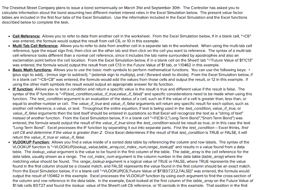
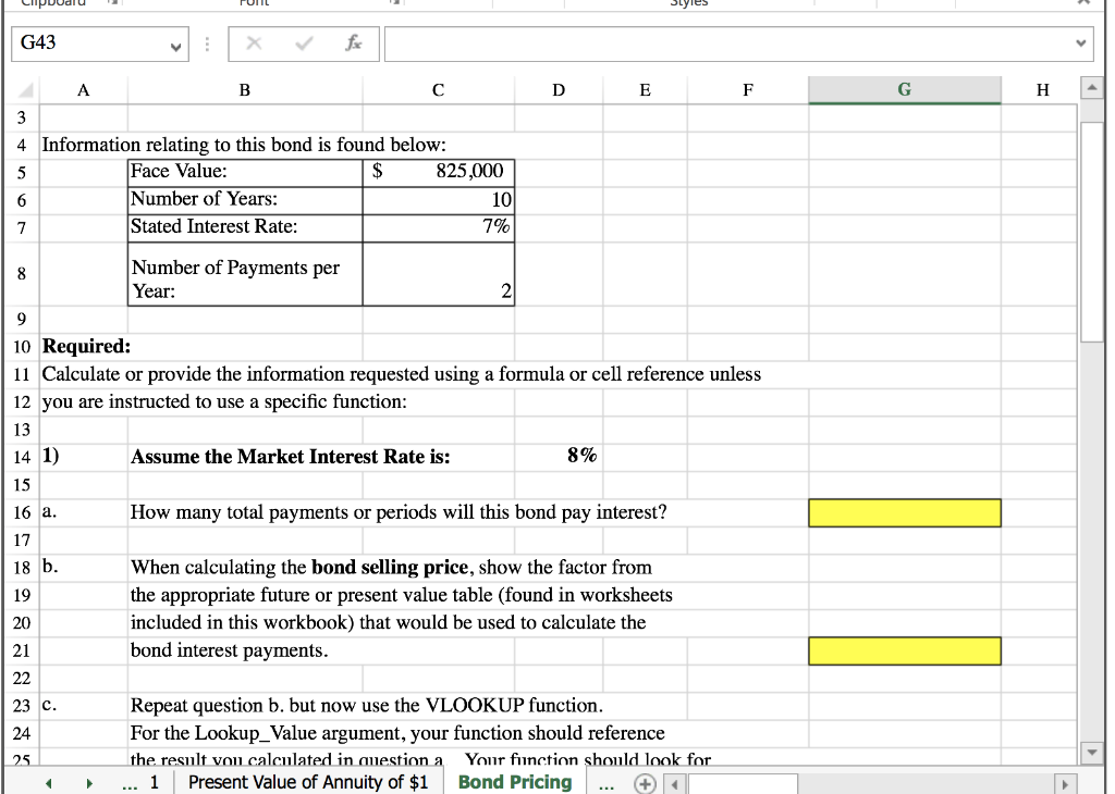
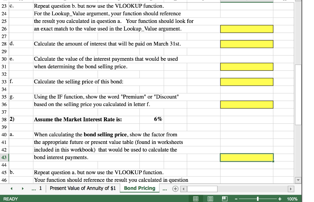
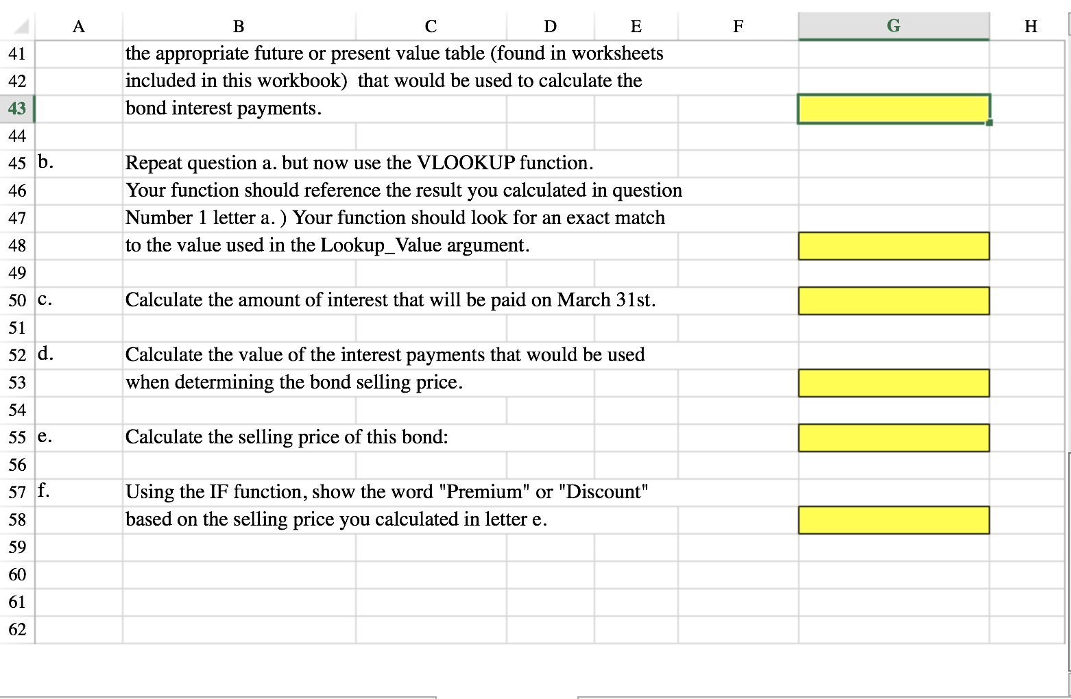
The Chestnut Street Company plans to issue a bond semiannually on March 31st and September 30th. The Controller has asked you to calculate information about the bond assuming two different market interest rates in the Excel Simulation below. The present value factor tables are included in the first four tabs of the Excel Simulation. Use the information included in the Excel Simulation and the Excel functions described below to complete the task. a . Cell Reference: Allows you to refer to data from another cell in the worksheet. From the Excel Simulation below, if in a blank cell, "=C6" was entered, the formula would output the result from cell C6, or 10 in this example. Multi-Tab Cell Reference: Allows you to refer to data from another cell in a separate tab in the worksheet. When using the multi-tab cell reference, type the equal sign first, then click on the other tab and then click on the cell you want to reference. The syntax of a multi-tab cell reference looks different than a normal cell reference, since it includes the tab name surrounded by apostrophes and also an exclamation point before the cell location. From the Excel Simulation below, if in a blank cell on the Sheet1 tab "='Future Value of $1'!C13" Below, was entered the formula would output the result from cell C13 in the Future Value of $1 tab, or 1.10462 in this example. Basic Math functions: Allows you to use the basic math symbols to perform mathematical functions. You can use the following keys: + (plus sign to add),- (minus sign to subtract), * (asterisk sign to multiply), and / (forward slash to divide). From the Excel Simulation below, if in a blank cell=C6+C8" was entered the formula would add the values from those cells and output the result, or 12 in this example. If using the other math symbols the result would output an appropriate answer for its function. IF function: Allows you to test a condition and return a specific value is the result is true and different value if the result is false. The syntax of the IF function is "=IF(test_condition, value_if_true,value_if_false)" and specific considerations need to be made when using this function. The test_condition argument is an evaluation of the status of a cell, such as if the value of a cell is greater than, less than, or equal to another number or cell. The value_if_true and value_if_false arguments will return any specific result for each option, such as nath tout anti another cell reference, a value, or text. Throughout the entire equation, if text is being used in the test_condition, value_if_true, or value_it_false arguments then the text itself should be entered in quotations so that Excel will recognize the text as a "string of text" nati instead of another function. From the Excel Simulation below, if in a blank cell =IF(C6>2,"Long-Term Bond","Short-Term Bond") was entered, the formula would output the result of the value_if_true since the test_condition would be result as true, or in this case the text "Long-Term Bond". Excel processes the IF function by separating it out into separate parts. First the test_condition - Excel thinks, find cell C6 and determine if the value is greater than 2. Once Excel determines if the result of that test_condition is TRUE or FALSE, it will return the value_if_true or value_it_false. VLOOKUP Function: Allows you find a value inside of a sorted data table by referencing the column and row labels. The syntax of the VLOOKUP function is "=VLOOKUP(lookup_value,table_array,col_index_num,range_lookup)" and results in a value found from a data table. The lookup_value argument is the value to be found in the first column of the table. The table_array is the cell reference for the data table, usually shown as a range. The col_index_num argument is the column number in the data table (table_array) where the matching value should be found. The range_lookup argument is a logical value of TRUE or FALSE, where TRUE represents the value found in the first column should be a closest match, and FALSE represents the value found in the first column should be an exact match. From the Excel Simulation below, if in a blank cell"=VLOOKUP(C6, 'Future Value of $1'!B3:T27,2,FALSE)" was entered, the formula would output the result of 1.10462 in this example. Excel processes the VLOOKUP function by using each argument to find the cross-section of the column and row reference in the data table. In the example, Excel looked at the first column of the table_array on the Future Value of $1 tab cells B3:127 and found the lookup value of the Sheet1 cell C6 reference. or 10 periods in this example. That position in the first G43 X A B D E F G H 3 4 Information relating to this bond is found below: 5 Face Value: 825,000 6 Number of Years: 10 7 Stated Interest Rate: 7% 8 Number of Payments per Year: 2 9 10 Required: 11 Calculate or provide the information requested using a formula or cell reference unless 12 you are instructed to use a specific function: 13 14 1) Assume the Market Interest Rate is: 8% 15 16 a. How many total payments or periods will this bond pay interest? 17 18 b. 19 When calculating the bond selling price, show the factor from the appropriate future or present value table (found in worksheets included in this workbook) that would be used to calculate the bond interest payments. 20 21 22 23 c. 24 Repeat question b. but now use the VLOOKUP function. For the Lookup_value argument, your function should reference the result you calculated in auestion a Your function should look for 1 Present Value of Annuity of $1 Bond Pricing 25 1 23 c. 24 Repeat question b. but now use the VLOOKUP function. For the Lookup_value argument, your function should reference the result you calculated in question a. Your function should look for an exact match to the value used in the Lookup_value argument. 25 26 27 28 d. Calculate the amount of interest that will be paid on March 31st. 29 30 e. Calculate the value of the interest payments that would be used when determining the bond selling price. 31 THE 32 33 f. Calculate the selling price of this bond: 34 35 g Using the IF function, show the word "Premium" or "Discount" based on the selling price you calculated in letter f. 36 37 38 2) Assume the Market Interest Rate is: 6% 39 40 a. 41 When calculating the bond selling price, show the factor from the appropriate future or present value table (found in worksheets included in this workbook) that would be used to calculate the bond interest payments. 42 43 44 45 b. 46 Repeat question a. but now use the VLOOKUP function. Your function should reference the result you calculated in question 1 Present Value of Annuity of $1 Bond Pricing READY 100% A B D F G H 41 E the appropriate future or present value table (found in worksheets included in this workbook) that would be used to calculate the bond interest payments. 42 43 44 45 b. 46 Repeat question a. but now use the VLOOKUP function. Your function should reference the result you calculated in question Number 1 letter a.) Your function should look for an exact match to the value used in the Lookup_Value argument. 47 . 48 49 50 c. Calculate the amount of interest that will be paid on March 31st. 51 52 d. Calculate the value of the interest payments that would be used when determining the bond selling price. 53 LITE 54 55 e. Calculate the selling price of this bond: 56 57 f. Using the IF function, show the word "Premium" or "Discount" based on the selling price you calculated in letter e. 58 59 60 61 62 The Chestnut Street Company plans to issue a bond semiannually on March 31st and September 30th. The Controller has asked you to calculate information about the bond assuming two different market interest rates in the Excel Simulation below. The present value factor tables are included in the first four tabs of the Excel Simulation. Use the information included in the Excel Simulation and the Excel functions described below to complete the task. a . Cell Reference: Allows you to refer to data from another cell in the worksheet. From the Excel Simulation below, if in a blank cell, "=C6" was entered, the formula would output the result from cell C6, or 10 in this example. Multi-Tab Cell Reference: Allows you to refer to data from another cell in a separate tab in the worksheet. When using the multi-tab cell reference, type the equal sign first, then click on the other tab and then click on the cell you want to reference. The syntax of a multi-tab cell reference looks different than a normal cell reference, since it includes the tab name surrounded by apostrophes and also an exclamation point before the cell location. From the Excel Simulation below, if in a blank cell on the Sheet1 tab "='Future Value of $1'!C13" Below, was entered the formula would output the result from cell C13 in the Future Value of $1 tab, or 1.10462 in this example. Basic Math functions: Allows you to use the basic math symbols to perform mathematical functions. You can use the following keys: + (plus sign to add),- (minus sign to subtract), * (asterisk sign to multiply), and / (forward slash to divide). From the Excel Simulation below, if in a blank cell=C6+C8" was entered the formula would add the values from those cells and output the result, or 12 in this example. If using the other math symbols the result would output an appropriate answer for its function. IF function: Allows you to test a condition and return a specific value is the result is true and different value if the result is false. The syntax of the IF function is "=IF(test_condition, value_if_true,value_if_false)" and specific considerations need to be made when using this function. The test_condition argument is an evaluation of the status of a cell, such as if the value of a cell is greater than, less than, or equal to another number or cell. The value_if_true and value_if_false arguments will return any specific result for each option, such as nath tout anti another cell reference, a value, or text. Throughout the entire equation, if text is being used in the test_condition, value_if_true, or value_it_false arguments then the text itself should be entered in quotations so that Excel will recognize the text as a "string of text" nati instead of another function. From the Excel Simulation below, if in a blank cell =IF(C6>2,"Long-Term Bond","Short-Term Bond") was entered, the formula would output the result of the value_if_true since the test_condition would be result as true, or in this case the text "Long-Term Bond". Excel processes the IF function by separating it out into separate parts. First the test_condition - Excel thinks, find cell C6 and determine if the value is greater than 2. Once Excel determines if the result of that test_condition is TRUE or FALSE, it will return the value_if_true or value_it_false. VLOOKUP Function: Allows you find a value inside of a sorted data table by referencing the column and row labels. The syntax of the VLOOKUP function is "=VLOOKUP(lookup_value,table_array,col_index_num,range_lookup)" and results in a value found from a data table. The lookup_value argument is the value to be found in the first column of the table. The table_array is the cell reference for the data table, usually shown as a range. The col_index_num argument is the column number in the data table (table_array) where the matching value should be found. The range_lookup argument is a logical value of TRUE or FALSE, where TRUE represents the value found in the first column should be a closest match, and FALSE represents the value found in the first column should be an exact match. From the Excel Simulation below, if in a blank cell"=VLOOKUP(C6, 'Future Value of $1'!B3:T27,2,FALSE)" was entered, the formula would output the result of 1.10462 in this example. Excel processes the VLOOKUP function by using each argument to find the cross-section of the column and row reference in the data table. In the example, Excel looked at the first column of the table_array on the Future Value of $1 tab cells B3:127 and found the lookup value of the Sheet1 cell C6 reference. or 10 periods in this example. That position in the first G43 X A B D E F G H 3 4 Information relating to this bond is found below: 5 Face Value: 825,000 6 Number of Years: 10 7 Stated Interest Rate: 7% 8 Number of Payments per Year: 2 9 10 Required: 11 Calculate or provide the information requested using a formula or cell reference unless 12 you are instructed to use a specific function: 13 14 1) Assume the Market Interest Rate is: 8% 15 16 a. How many total payments or periods will this bond pay interest? 17 18 b. 19 When calculating the bond selling price, show the factor from the appropriate future or present value table (found in worksheets included in this workbook) that would be used to calculate the bond interest payments. 20 21 22 23 c. 24 Repeat question b. but now use the VLOOKUP function. For the Lookup_value argument, your function should reference the result you calculated in auestion a Your function should look for 1 Present Value of Annuity of $1 Bond Pricing 25 1 23 c. 24 Repeat question b. but now use the VLOOKUP function. For the Lookup_value argument, your function should reference the result you calculated in question a. Your function should look for an exact match to the value used in the Lookup_value argument. 25 26 27 28 d. Calculate the amount of interest that will be paid on March 31st. 29 30 e. Calculate the value of the interest payments that would be used when determining the bond selling price. 31 THE 32 33 f. Calculate the selling price of this bond: 34 35 g Using the IF function, show the word "Premium" or "Discount" based on the selling price you calculated in letter f. 36 37 38 2) Assume the Market Interest Rate is: 6% 39 40 a. 41 When calculating the bond selling price, show the factor from the appropriate future or present value table (found in worksheets included in this workbook) that would be used to calculate the bond interest payments. 42 43 44 45 b. 46 Repeat question a. but now use the VLOOKUP function. Your function should reference the result you calculated in question 1 Present Value of Annuity of $1 Bond Pricing READY 100% A B D F G H 41 E the appropriate future or present value table (found in worksheets included in this workbook) that would be used to calculate the bond interest payments. 42 43 44 45 b. 46 Repeat question a. but now use the VLOOKUP function. Your function should reference the result you calculated in question Number 1 letter a.) Your function should look for an exact match to the value used in the Lookup_Value argument. 47 . 48 49 50 c. Calculate the amount of interest that will be paid on March 31st. 51 52 d. Calculate the value of the interest payments that would be used when determining the bond selling price. 53 LITE 54 55 e. Calculate the selling price of this bond: 56 57 f. Using the IF function, show the word "Premium" or "Discount" based on the selling price you calculated in letter e. 58 59 60 61 62