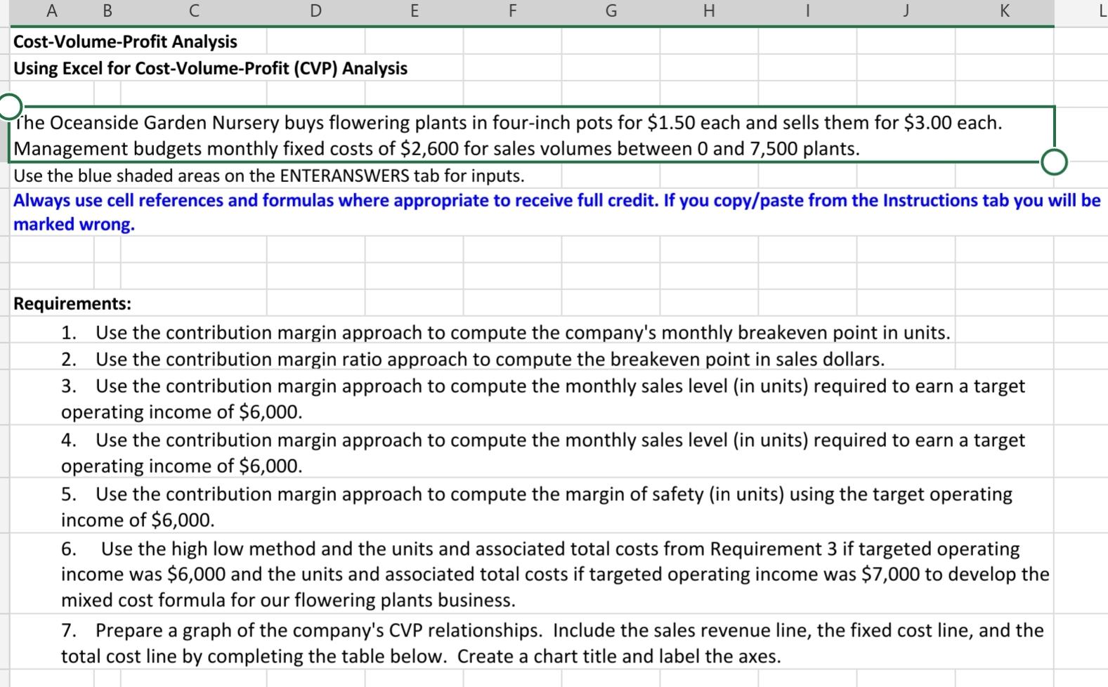
The oceanside garden nursery buys flowering plants In 4-inch pots for $1.50 each and sells them for $3.00 each. Management budgets monthly fixed costs of $2600 for sales volume between 0 and 7500 plants

Please include formula also!!

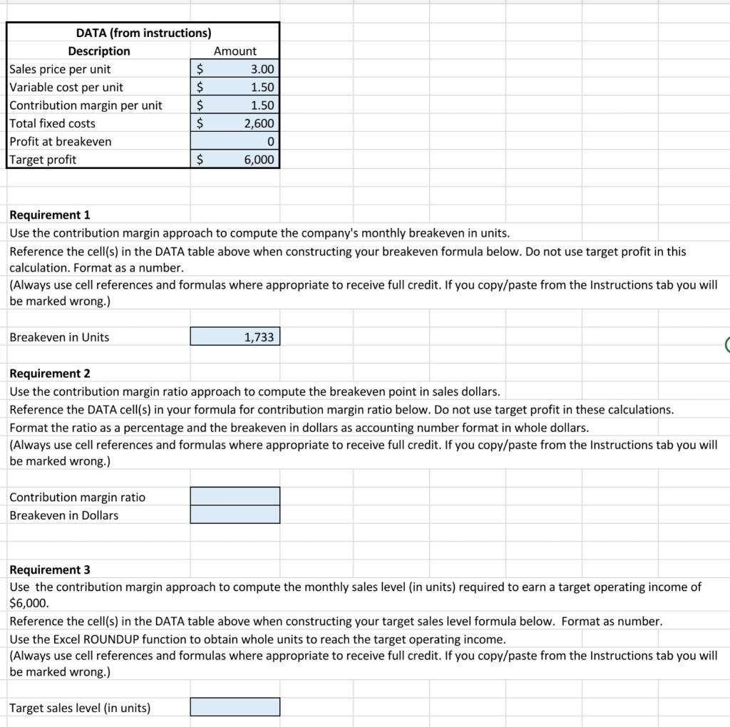
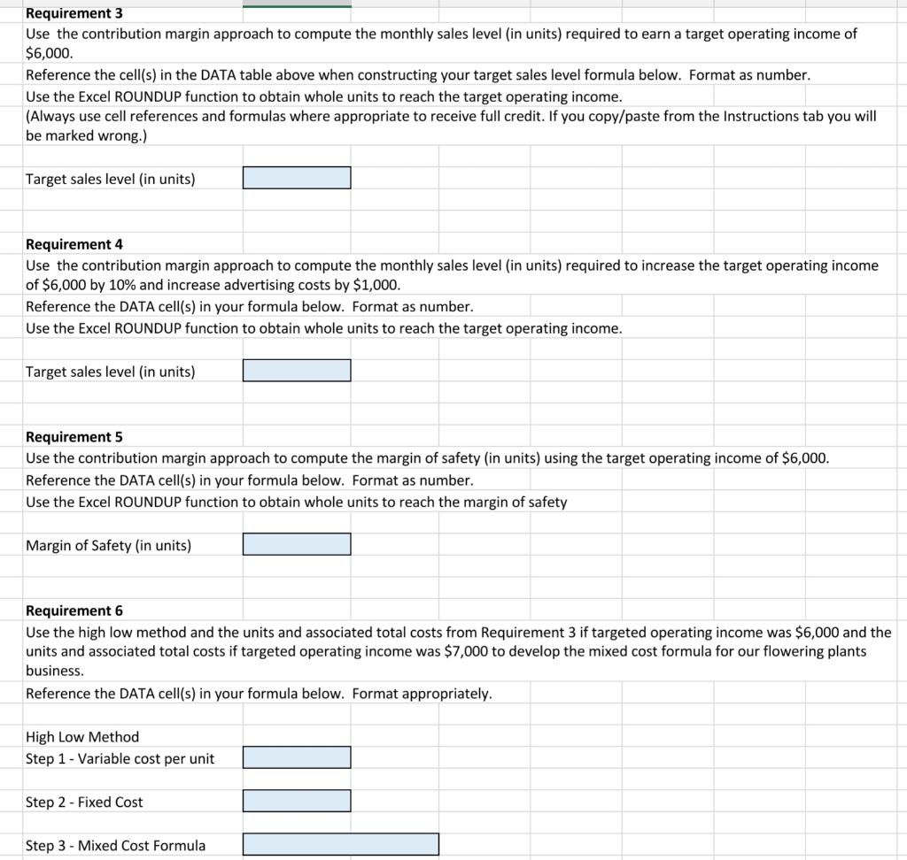
A B C D E F G H K L Cost-Volume-Profit Analysis Using Excel for Cost-Volume-Profit (CVP) Analysis The Oceanside Garden Nursery buys flowering plants in four-inch pots for $1.50 each and sells them for $3.00 each. Management budgets monthly fixed costs of $2,600 for sales volumes between 0 and 7,500 plants. Use the blue shaded areas on the ENTERANSWERS tab for inputs. Always use cell references and formulas where appropriate to receive full credit. If you copy/paste from the Instructions tab you will be marked wrong. Requirements: 1. Use the contribution margin approach to compute the company's monthly breakeven point in units. 2. Use the contribution margin ratio approach to compute the breakeven point in sales dollars. 3. Use the contribution margin approach to compute the monthly sales level (in units) required to earn a target operating income of $6,000. 4. Use the contribution margin approach to compute the monthly sales level (in units) required to earn a target operating income of $6,000. 5. Use the contribution margin approach to compute the margin of safety (in units) using the target operating income of $6,000. 6. Use the high low method and the units and associated total costs from Requirement 3 if targeted operating income was $6,000 and the units and associated total costs if targeted operating income was $7,000 to develop the mixed cost formula for our flowering plants business. 7. Prepare a graph of the company's CVP relationships. Include the sales revenue line, the fixed cost line, and the total cost line by completing the table below. Create a chart title and label the axes. DATA (from instructions) Description Amount Sales price per unit $ 3.00 Variable cost per unit $ 1.50 Contribution margin per unit $ 1.50 Total fixed costs $ 2,600 Profit at breakeven 0 Target profit $ 6,000 Requirement 1 Use the contribution margin approach to compute the company's monthly breakeven in units. Reference the cell(s) in the DATA table above when constructing your breakeven formula below. Do not use target profit in this calculation. Format as a number. (Always use cell references and formulas where appropriate to receive full credit. If you copy/paste from the Instructions tab you will be marked wrong.) Breakeven in Units 1,733 Requirement 2 Use the contribution margin ratio approach to compute the breakeven point in sales dollars. Reference the DATA cell(s) in your formula for contribution margin ratio below. Do not use target profit in these calculations. Format the ratio as a percentage and the breakeven in dollars as accounting number format in whole dollars. (Always use cell references and formulas where appropriate to receive full credit. If you copy/paste from the Instructions tab you will be marked wrong.) Contribution margin ratio Breakeven in Dollars Requirement 3 Use the contribution margin approach to compute the monthly sales level (in units) required to earn a target operating income of $6,000. Reference the cell(s) in the DATA table above when constructing your target sales level formula below. Format as number. Use the Excel ROUNDUP function to obtain whole units to reach the target operating income. (Always use cell references and formulas where appropriate to receive full credit. If you copy/paste from the Instructions tab you will be marked wrong.) Target sales level (in units) Requirement 3 Use the contribution margin approach to compute the monthly sales level (in units) required to earn a target operating income of $6,000. Reference the cell(s) in the DATA table above when constructing your target sales level formula below. Format as number. Use the Excel ROUNDUP function to obtain whole units to reach the target operating income. (Always use cell references and formulas where appropriate to receive full credit. If you copy/paste from the Instructions tab you will be marked wrong.) Target sales level (in units) Requirement 4 Use the contribution margin approach to compute the monthly sales level (in units) required to increase the target operating income of $6,000 by 10% and increase advertising costs by $1,000. Reference the DATA cell(s) in your formula below. Format as number. Use the Excel ROUNDUP function to obtain whole units to reach the target operating income. Target sales level in units) Requirement 5 Use the contribution margin approach to compute the margin of safety (in units) using the target operating income of $6,000. Reference the DATA cell(s) in your formula below. Format number. Use the Excel ROUNDUP function to obtain whole units to reach the margin of safety Margin of Safety (in units) Requirement 6 Use the high low method and the units and associated total costs from Requirement 3 if targeted operating income was $6,000 and the units and associated total costs if targeted operating income was $7,000 to develop the mixed cost formula for our flowering plants business. Reference the DATA cell(s) in your formula below. Format appropriately. High Low Method Step 1 - Variable cost per unit Step 2 - Fixed Cost Step 3 - Mixed Cost Formula