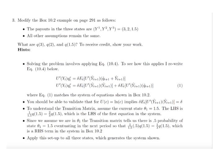
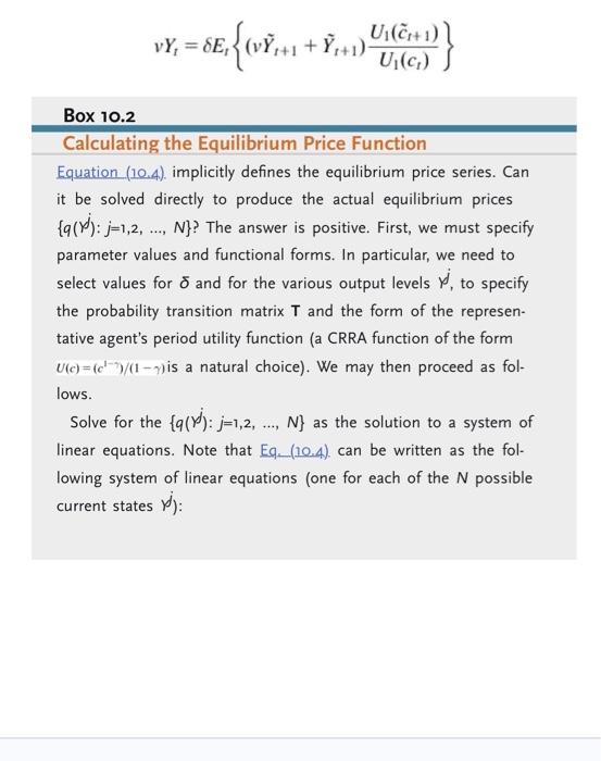
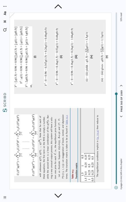
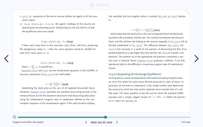
- The payouts in the three states are (Y1,Y2,Y3)=(3,2,1.5) - All other assumptions remain the same. What are q(3),q(2), and q(1.5) ? To receive credit, show your work. Iints: - Solving the problem involves applying Eq. (10.4). To see how this applies I rewrite Eq. (10.4) below. U(Yt)qi=Et[U(Y~t+1)(q^t+1+Y~t+1)]U(Yt)qi=Et[U(Y^t+1)(Y~t+1)]+Et[U(Y~t+1)(q~t+1)] where Eq. (1) matches the system of equations shown in Box 10.2. - You should be able to validate that for U(c)=ln(c) implies Et[U(Y~t+1)(Y~t+1)]= - To understand the Transition Matrix, assume the current state 1=1.5. The LHS is 1.51q(1.5)=32q(1.5), which is the LHS of the first equation in the system. - Since we assume we are in 1 the Transition matrix tells us there is . 5 probability of state 1=1.5 eventuating in the next period so that 1.51(.5)q(1.5)=31q(1.5), which is a RHS term in the system in Box 10.2 - Apply this set-up to all three states, which generates the system shown. vYt=Et{(vY~t+1+Y~t+1)U1(ct)U1(c~t+1)} Box 10.2 Calculating the Equilibrium Price Function Equation (10.4). implicitly defines the equilibrium price series. Can it be solved directly to produce the actual equilibrium prices {q(j):j=1,2,,N} ? The answer is positive. First, we must specify parameter values and functional forms. In particular, we need to select values for and for the various output levels , to specify the probability transition matrix T and the form of the representative agent's period utility function (a CRRA function of the form U(c)=(c1h)/(1) is a natural choice). We may then proceed as follows. Solve for the {q():j=1,2,,N} as the solution to a system of linear equations. Note that Eq. (10.4). can be written as the following system of linear equations (one for each of the N possible current states j ): S SCRIBD U1(Y)q(YI)=j=1NUU1(Y)+=1N1jU1(Yj)q(Y)Y1:22q(1.5)=0.96+0.96{41q(1.5)+11q(1)+tq(0.5)}2:q(1)=0.96+0.96{61q(1.5)+21q(1)+21q(0.5)}3:2q(0.5)=0.96+0.96{61q(1.5)+41q(1)+1q(0.5)}U1(YN)q(YN)=j=1NNU1(Y)Yd+j=1NNU1(Y)q(Y) with unknowns a(m),q(r),44[N). Note that for each of there equations, the fint term on the RHS is rimply a number. while the second term is a linear combination of the q(h)s. Ean. y:0=0.960.3474(1.5)+0.24q(1)+0.48q(0.5) ring a very unusual output process, this sstem will have a solu. Let us illustrate. Suppese U(c)=ln(q),0.96 and (n,y,n, y2:0=0.96+0.16q(1.5)0.52q(1)+0.48q(0.5) M7-(1.5, 1, 0.5) - an exaggeration of boam, nomtal, and depersison (ii) times. The transtion matris is when to be as found in Table say. Table 10.3 y3:0=0.96+0.16q(1.5)+0.24q(1)1.04q(0.5) Transition matrix (iii) (i) - (ii) yields : q(1.5)=6.5007q(1)=1.5 op (1) (iv) The equilibrium coodition implicit in Eu.fical then reduce to (ii) - (iii) gives ;q(0.5)=13t026(1)=1/2q(1) ii. ctYE, .e, ownership of the entire security entitles the agent to all the econrisk neutrality and the marginal ueility is constant {U11=0). Eq. (ma.6\} reduces omy's output: bo optimal given the prevailing peices. Substituting (ii) into (ii) informs us that the equilbrium price must satisfy which states that the stock price is the sum of empected future dividends discounted an the (constanf) risk-free rate. The imtuitive link between the disceunt factor and the riskifree rate leading to the second inequality in Eq. (ia.3) will be If there were many fisms in this economy-say f firms, with fiem j producing formally established in Eq. (to.9). The diference between Los. (roig and the (exogenous) output fk - then the same equation would be satisfied for (go.7) is the necessity, in a world of risk aversion, of discounting the flow of each fiem's stoek price, if l.e. pected dividends at a rate higher than the riskfree rate, so as to include a risk. premium, The question as to the appropriate risk premium coristitutes a cen. tal issue in financial theory. Eaualien. the.6t proposes a definite, if not fully operational (due to the difficulty in measuring marginal rates of substitution). where 6=2rp in equilibrium. answer. Louatiana (10.4) and (10.5) are the fundamental equations of the CCAPMZ A recursive substitution of Eq. (10.2) imo itself yields: 10.3-2 Interpreting the Exchange Equilibrium To bring about a closer correspondence with traditional asset pricing formulas. we must firt relate the asset prices derived previously to rates of return, in particulac we will want to understand, in this model conteat, what determines establishing the stock price is the sum of all expected disceunted future the amount by which the risky asset's expected return exceeds that of a risk. dividends. Equation (io.te) resembles the standard discounting formula of ele. free asset. This basic question is also the one for which the standand CAPM mentary finance, but for the impertant observation that dircounting akes place using the intertemporal marginal rates of substitution defined on the con. to i+1 tetum for secutity j as sumption sequence of the representative agent. If the utility function displays A papes (4 min) leh in this chapter PAGE 545 OF 1069