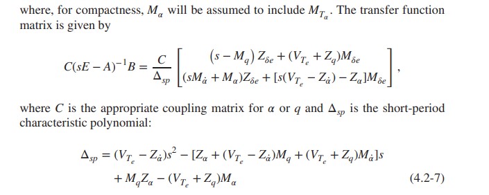
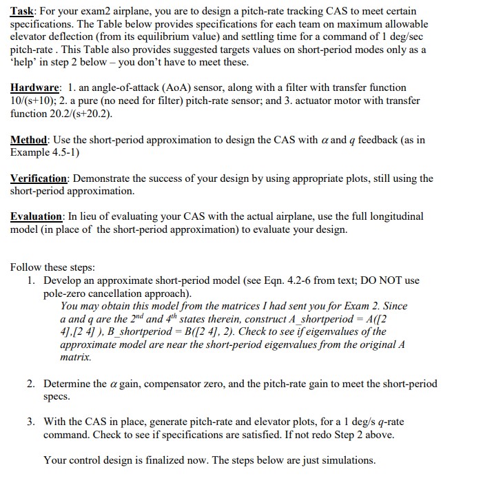
The Short-Period Approximation The short-period approximation obtained from (4.2-5) is [VTe Zi 0 -M Za VTe+Zq Zse (4.2-6) + Mse = Ma Ma where, for compactness, M will be assumed to include Mr. The transfer function matrix is given by C(SE-A)-B= (s-Ma) Zse+(VT +ZqMse - sp [(SM+Ma)Zse + [s(VT Z) Za]Me where C is the appropriate coupling matrix for a or q and Asp is the short-period characteristic polynomial: Asp = (VT-Za)s - [Za + (Vr Z)Mq + (Vr+Zq)M]s +MqZa - (VT+Zq)Ma (4.2-7) Task: For your exam2 airplane, you are to design a pitch-rate tracking CAS to meet certain specifications. The Table below provides specifications for each team on maximum allowable elevator deflection (from its equilibrium value) and settling time for a command of 1 deg/sec pitch-rate. This Table also provides suggested targets values on short-period modes only as a 'help' in step 2 below - you don't have to meet these. Hardware: 1. an angle-of-attack (AOA) sensor, along with a filter with transfer function 10/(s+10); 2. a pure (no need for filter) pitch-rate sensor; and 3. actuator motor with transfer function 20.2/(s+20.2). Method: Use the short-period approximation to design the CAS with a and q feedback (as in Example 4.5-1) Verification: Demonstrate the success of your design by using appropriate plots, still using the short-period approximation. Evaluation: In lieu of evaluating your CAS with the actual airplane, use the full longitudinal model (in place of the short-period approximation) to evaluate your design. Follow these steps: 1. Develop an approximate short-period model (see Eqn. 4.2-6 from text; DO NOT use pole-zero cancellation approach). You may obtain this model from the matrices I had sent you for Exam 2. Since a and q are the 2nd and 4th states therein, construct A_shortperiod = A([2 4],[24]), B_shortperiod = B([24], 2). Check to see if eigenvalues of the approximate model are near the short-period eigenvalues from the original A matrix. 2. Determine the a gain, compensator zero, and the pitch-rate gain to meet the short-period specs. 3. With the CAS in place, generate pitch-rate and elevator plots, for a 1 deg/s q-rate command. Check to see if specifications are satisfied. If not redo Step 2 above. Your control design is finalized now. The steps below are just simulations. specification suggested values max short- shot-period settling elevator (deg) period damped freq time (sec) damping (rad/s) 2.00 5.00 0.70 6.00 4. Repeat Step 3 above with the approximate model replaced by the full linearized longitudinal model. You will now have four airplane states. Plot all the airplane states and elevator movement. Make appropriate observation.