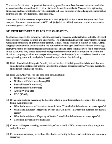
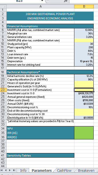
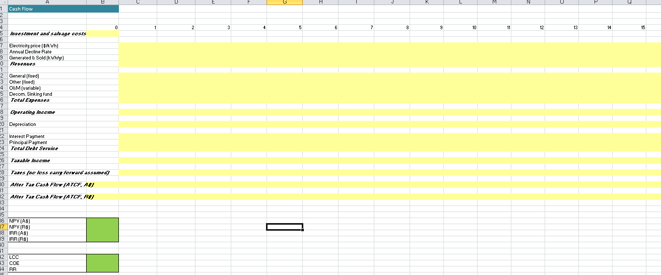
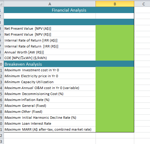
The spreadsheet that accompanies this case study provides some baseline cost estimates and other assumptions that you will use to create a discounted cash flow analysis. Many of the engineering. financing, and tax complexities have been simplified. Cost estimates are based on public information sources and are for educational purposes only. Note that all dollar amounts are provided in REAL (R3) dollars for Year 0. For your cash flow analysis, these nust be converted to ACTUAL ( A$ ) dollars. All A$ amounts should be assumed to vary with general inflation. STUDENT DELIVERABLES FOR THE CASE STUDY Students are expected to produce a realistic engineering economy analysis that includes the effects of taxes and depreciation, inflation and uncertainty. The analysis should all be in excel with the opening worksheet containing an Introduction (approx. 1 page) neatly typed in a textbox in excel. Using languape that would be understandable to a non-technical manager, briefly describe the tectunology and why it merits an engineering economic analysis. The use of the template excel file is encouraged. If you wish, you may create additional background information and assumptions related to the: fictitious company, markets and competitive strategy. Let the rest of your worksheets describe how an engineering economic analysis is done with emphasis an the following: [1] Cash Flow Model. Complete/modify the spreadsheet template provided. Make sure that your spreadsheet model is constructed to facilitate the analyses described below. You may modify the spreadsheet template as needed. (2) Base Case Analysis. For the base case data, calculate: - Net Present Value (solved using A3) - Net Present Value (solved using R\$) - Internal Rate of Return (AS) - Internal Rate of Return (R\$) - Anrual Warth (RS) - COE(3/kWh) [3] Break-even analysis. Assuming the baseline values in your financial model, answer the following break-even questions: - What is the maximum "Investment cast in Year 0 " at which this business can make a profit? - What is the minimum" Electricity price in Year 0(5/kWh)at which this business can make a profit? - What is the minimum "Capacity utilization" at which this business can make a profit? - Canduct a payback period analysis. [4] Create a spider plot showing the sensitivity of the actual $ NPV to irvestment, electricity price and utilization. [5] Perform ascenarioanalysis anthree likelihoodsincluding the base-case, best-case and worst-case screnarios. \begin{tabular}{|c|c|c|c|} \hline \multirow{2}{*}{1} & \multicolumn{2}{|r|}{ A } & B \\ \hline & & & \\ \hline 2 & \multicolumn{3}{|c|}{200 MW GEOTHERMAL POWER PLANT } \\ \hline 3 & \multicolumn{3}{|c|}{ ENGINEERING ECONOMIC ANALYSIS } \\ \hline \multicolumn{4}{|l|}{4} \\ \hline 5 & \multicolumn{3}{|c|}{ Financial Assumptions } \\ \hline 6 & \multicolumn{2}{|c|}{ MARR (A\$ ater-tan, combined market rate) } & 13.00% \\ \hline 7 & \multicolumn{2}{|l|}{ Marginal tau rate } & 36% \\ \hline 8 & \multicolumn{2}{|c|}{ General inflation rate } & 3.20% \\ \hline 9 & \multicolumn{2}{|c|}{ MARR (R\$ after-tax, combined market rate) } & \\ \hline 10 & \multicolumn{2}{|l|}{ Study period (yrs) } & 30 \\ \hline 11 & \multicolumn{2}{|l|}{ Plant capacity (MW') } & 200 \\ \hline 12 & \multicolumn{2}{|l|}{ Debt \% } & 60% \\ \hline 13 & \multicolumn{2}{|l|}{ Loan interest rate } & 7.0% \\ \hline 14 & \multicolumn{2}{|l|}{ Debt term (yrs.) } & 15 \\ \hline 15 & \multicolumn{2}{|l|}{ Depreciation } & 10 years SL \\ \hline 16 & \multicolumn{2}{|c|}{ Interest rate for sinking fund } & 3.20% \\ \hline \multicolumn{4}{|c|}{17} \\ \hline 18 & \multicolumn{3}{|c|}{ Technical Assumptions* } \\ \hline 19 & \multicolumn{2}{|c|}{ Initial harmonic decline rate (\%) } & 12.2% \\ \hline 20 & \multirow{2}{*}{\multicolumn{2}{|c|}{\begin{tabular}{l} Capacity utilization (\% of 200MW ) \\ Hours of operation per year \end{tabular}}} & 90% \\ \hline 21 & & & \\ \hline 22 & \multicolumn{2}{|c|}{ Generated \& Sold (in Yr 0) (MWh) } & \\ \hline 23 & \multicolumn{2}{|c|}{ Investment cost in Yr 0 (Formulation) } & \\ \hline 24 & \multicolumn{2}{|c|}{ Investment cost in Yr 0} & $406,130,175 \\ \hline 25 & \multicolumn{2}{|c|}{ Annual general expenses (fixed) } & $820,000 \\ \hline 26 & Other costs [fined) & & $518,000 \\ \hline 27 & Annual O\&M [\$\$k & & $0.0309 \\ \hline 28 & Decommissioning & cos% & 10% \\ \hline 29 & End-of-life decom & Tissioning cost & \\ \hline 30 & Decommissioning & cost in Yr30 & \\ \hline 31 & Electricity price in & r 0 [\$\$k'Wh] & $0.0808 \\ \hline \begin{tabular}{l} 32 \\ 33 \end{tabular} & (all initial monetar & values are provided in R\$ for Year 0 ) & \\ \hline 34 & NPV & & \\ \hline 35 & IRR (AS) & & \\ \hline 36 & IRR(RS) & & \\ \hline 37 & & & \\ \hline 38 & & & \\ \hline 39 & & & \\ \hline 40 & & & \\ \hline 41 & Sensitivity Table & & \\ \hline 42 & & & \\ \hline 43 & & & \\ \hline 44 & & & \\ \hline 141 & & Parameters CashFlow & Breakeven \\ \hline \end{tabular} Cash Flow hyestment abo'sabage costs Electricity price (\$\$k'wh) Annual Decline Rate Generated \& Sold (k'Whryr) Beyesues General (fixed) Dther [Fined] D (uariable) Decom. Sinking fund Toral Espenses Gperating hecome Depreciation Interest Payment Principal Payment Toral Debt Seryice Tasable bcowe Tases (oo hoss carr fortard assumed) AfIer Tas Casd Flow (ATCF. At) AfIer Tas Casd Flow (ATCF. BS) NPV [A$] NPV(R$) IRR [A$) IRR [R$ ) LCC COE RR