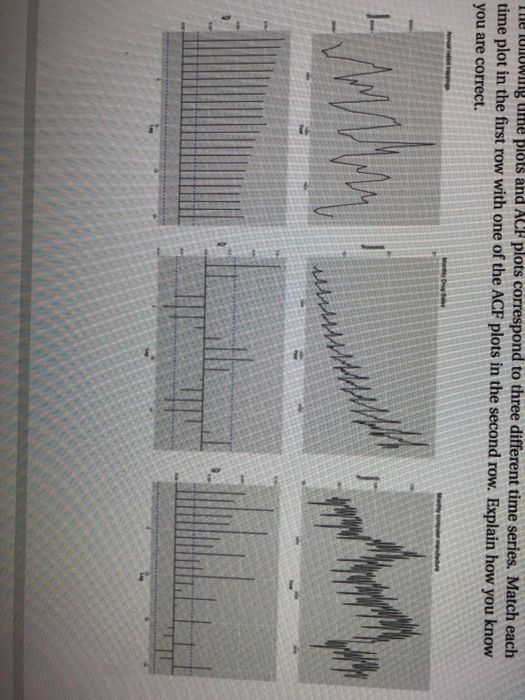
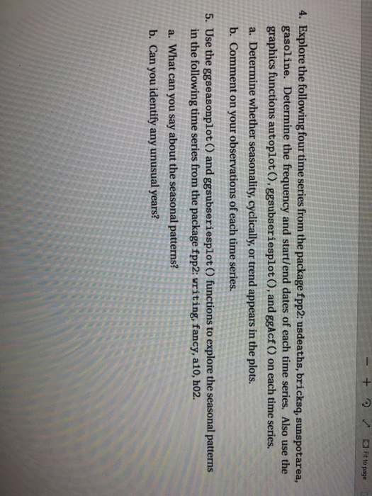
The unwing ume plots and ACF plots correspond to three different time series. Match each time plot in the first row with one of the ACF plots in the second row. Explain how you know you are correct. - + Fit to page D 4. Explore the following four time series from the package fpp2: usdeaths, bricks, sunspotarea, gasoline. Determine the frequency and start/end dates of each time series. Also use the graphics functions autoplot(), ggsubseriesplot(), and ggAcf () on each time series. a. Determine whether seasonality, cyclically, or trend appears in the plots. b. Comment on your observations of each time series. 5. Use the ggseasonplot() and ggsubseriesplot() functions to explore the seasonal patterns in the following time series from the package fpp2: writing, fancy, a10, h02. a. What can you say about the seasonal patterns? b. Can you identify any unusual years? The unwing ume plots and ACF plots correspond to three different time series. Match each time plot in the first row with one of the ACF plots in the second row. Explain how you know you are correct. - + Fit to page D 4. Explore the following four time series from the package fpp2: usdeaths, bricks, sunspotarea, gasoline. Determine the frequency and start/end dates of each time series. Also use the graphics functions autoplot(), ggsubseriesplot(), and ggAcf () on each time series. a. Determine whether seasonality, cyclically, or trend appears in the plots. b. Comment on your observations of each time series. 5. Use the ggseasonplot() and ggsubseriesplot() functions to explore the seasonal patterns in the following time series from the package fpp2: writing, fancy, a10, h02. a. What can you say about the seasonal patterns? b. Can you identify any unusual years