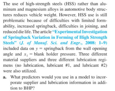
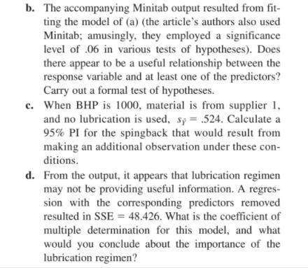
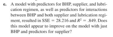
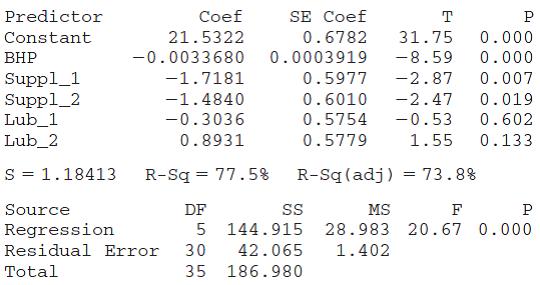
The use of high-strength steels (HSS) rather than alu- minum and magnesium alloys in automotive body struc- tures reduces vehicle weight. However, HSS use is still problematic because of difficulties with limited form- ability, increased springback, difficulties in joining, and reduced die life. The article "Experimental Investigation of Springback Variation in Forming of High Strength Steels" (J. of Manuf. Sci. and Engr., 2008: 1-9) included data on y = springback from the wall opening angle and x, = blank holder pressure. Three different material suppliers and three different lubrication regi- mens (no lubrication, lubricant #1, and lubricant #2) were also utilized. a. What predictors would you use in a model to incor- porate supplier and lubrication information in addi- tion to BHP? b. The accompanying Minitab output resulted from fit- ting the model of (a) (the article's authors also used Minitab; amusingly, they employed a significance level of .06 in various tests of hypotheses). Does there appear to be a useful relationship between the response variable and at least one of the predictors? Carry out a formal test of hypotheses. c. When BHP is 1000, material is from supplier 1, and no lubrication is used, sy = .524. Calculate a 95% PI for the spingback that would result from making an additional observation under these con- ditions. d. From the output, it appears that lubrication regimen may not be providing useful information. A regres- sion with the corresponding predictors removed resulted in SSE = 48.426. What is the coefficient of multiple determination for this model, and what would you conclude about the importance of the lubrication regimen? e. A model with predictors for BHP, supplier, and lubri- cation regimen, as well as predictors for interactions between BHP and both supplier and Ilubrication regi- ment, resulted in SSE = 28.216 and R = .849. Does this model appear to improve on the model with just BHP and predictors for supplier? Predictor Coef SE Coef T Constant 21.5322 0.6782 31.75 0.000 -0.0033680 0.0003919 -8.59 0.000 Suppl_1 Suppl_2 Lub_1 Lub_2 -1.7181 0.5977 -2.87 0.007 -1.4840 0.6010 -2.47 0.019 -0.3036 0.5754 -0.53 0.602 0.8931 0.5779 1.55 0.133 S = 1.18413 R-Sq = 77.5% R-Sq (adj) = 73.8% Source DF MS F Regression 5 144.915 28.983 20.67 0.000 Residual Error 30 42.065 1.402 Total 35 186.980