This coursework requires should be a technical report format that discusses the managerial problem, the results, and their implications and recommendations for improvement must be made.

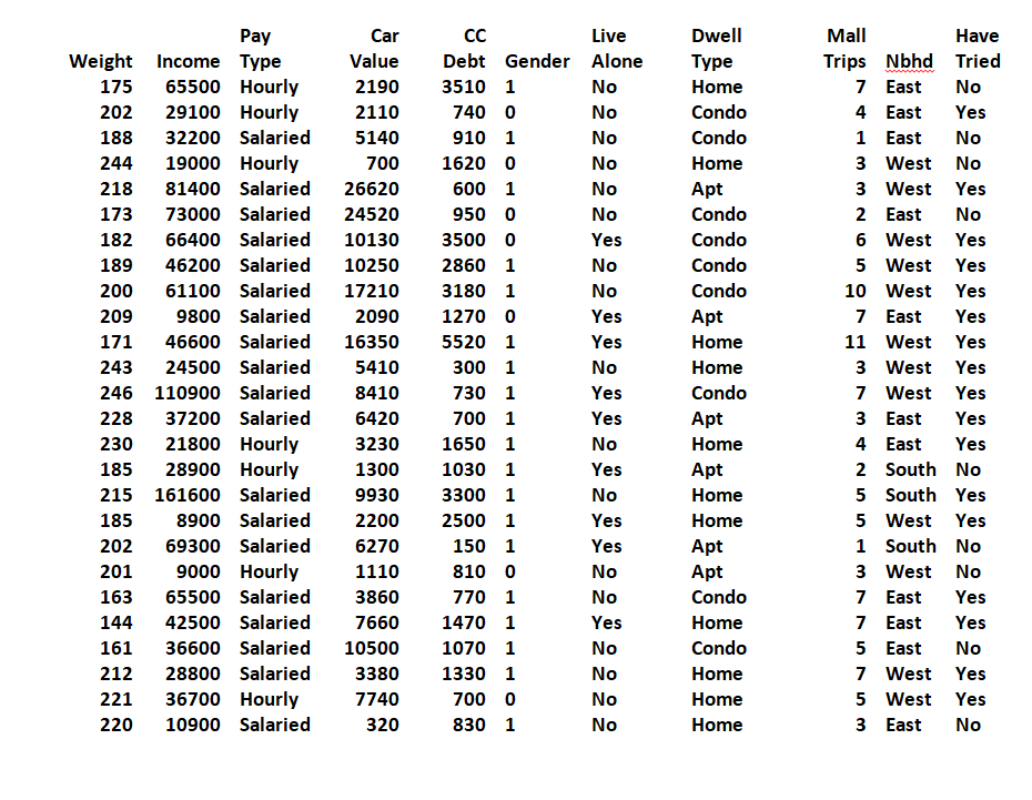
The data file is called Lasagna Triers.xlsx. Based on this data, you are required to identify a management decision problem or a research question - that can be addressed using the variables in the data. You can use Excel to conduct an analytic for the problem, elaboration on the results, and make managerial implications.

Introduction- In this section, you will identify your research question - based on the Excel Data. It is important to give reasons for why you think it's interesting to explore such question.

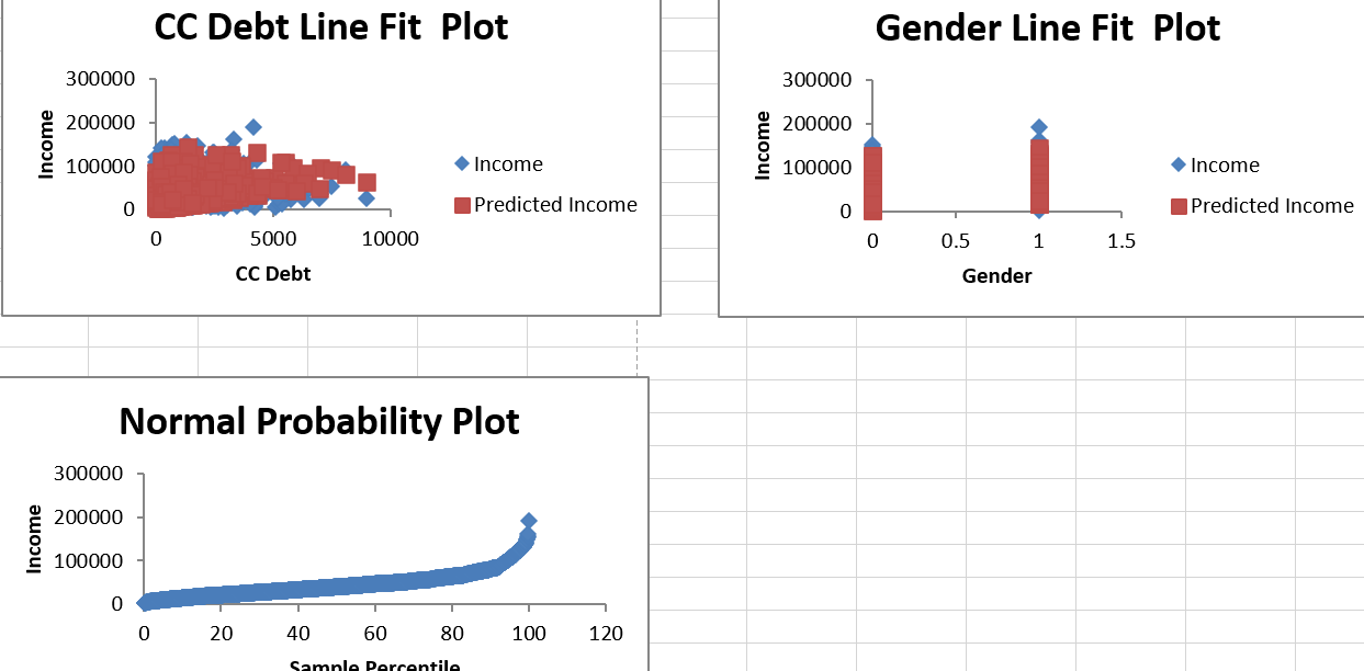
Descriptive analysis- Import the raw data to the database, make sure it imported correctly, identify the main tables and relationships between, produce relevant visualizations.

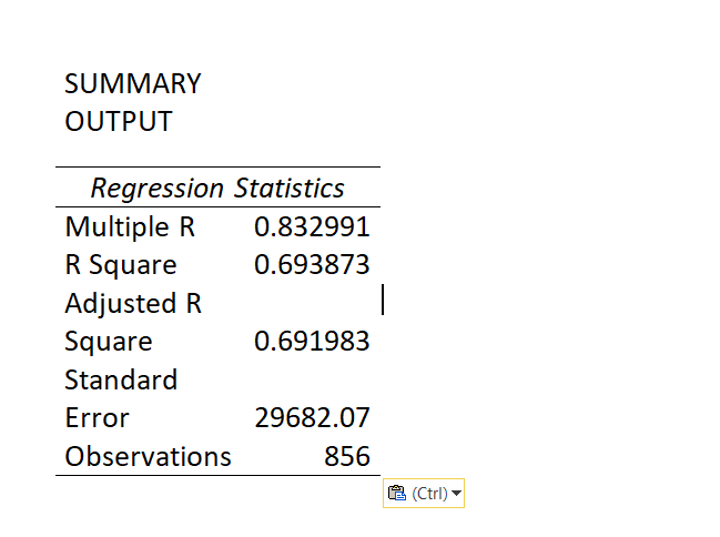
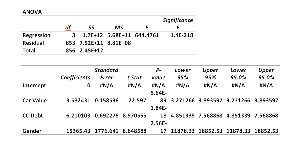
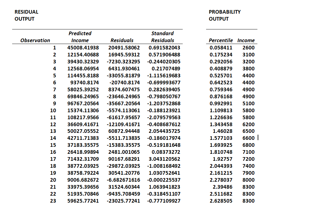
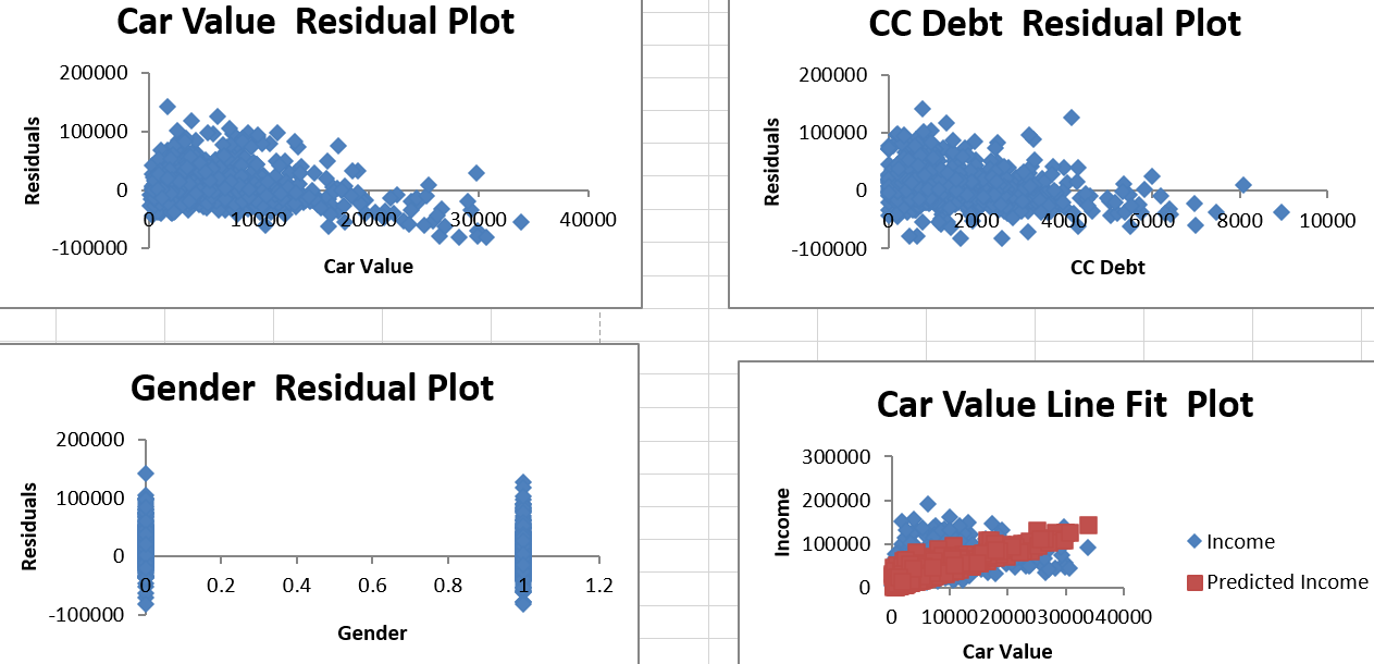
Regression analytics- Using appropriate regression models to address the managerial problem

Managerial interpretations and implications- It's important to provide some discussion on your findings. For example, if you find that the coefficient for men is positive i.e., men have higher salary than women. You can explain why this might be the case. Also, it's good idea to make references to academic studies that may or may not support your results.

Conclusion/ recommendations- What would be the managerial implications for your results? For example, if men have higher salary then women, what would you like to recommend either from the government's policy perspective, and/or from the firm's HR practices perspective.

Data: https://www.coursehero.com/textbook-solutions/we-used-the-lasagna-triers-xlsx-file-in-this-section-to-show-how-pivot-tables-can-help-9780357109953-631/Chapter-3-Problem-46-1072532/

Book: https://books.google.co.uk/books?id=pSEADAAAQBAJ&pg=PA125&lpg=PA125&dq=Weight%09Income%09Pay+Type%09Car+Value%09CC+Debt%09Gender%09Live+Alone%09Dwell+Type%09Mall+Trips%09Nbhd%09Have+Tried+175%0965500%09Hourly%092190%093510%091%09No%09Home%097%09East%09No+202%0929100%09Hourly%092110%09740%090%09No%09Condo%094%09East%09Yes+188%0932200%09Salaried%095140%09910%091%09No%09Condo%091%09East%09No+244%0919000%09Hourly%09700%091620%090%09No%09Home%093%09West%09No+218%0981400%09Salaried%0926620%09600%091%09No%09Apt%093%09West%09Yes+173%0973000%09Salaried%0924520%09950%090%09No%09Condo%092%09East%09No+182%0966400%09Salaried%0910130%093500%090%09Yes%09Condo%096%09West%09Yes+189%0946200%09Salaried%0910250%092860%091%09No%09Condo%095%09West%09Yes+200%0961100%09Salaried%0917210%093180%091%09No%09Condo%0910%09West%09Yes+209%099800%09Salaried%092090%091270%090%09Yes%09Apt%097%09East%09Yes+171%0946600%09Salaried%0916350%095520%091%09Yes%09Home%0911%09West%09Yes+243%0924500%09Salaried%095410%09300%091%09No%09Home%093%09West%09Yes+246%09110900%09Salaried%098410%09730%091%09Yes%09Condo%097%09West%09Yes+228%0937200%09Salaried%096420%09700%091%09Yes%09Apt%093%09East%09Yes+230%0921800%09Hourly%093230%091650%091%09No%09Home%094%09East%09Yes+185%0928900%09Hourly%091300%091030%091%09Yes%09Apt%092%09South%09No+215%09161600%09Salaried%099930%093300%091%09No%09Home%095%09South%09Yes+185%098900%09Salaried%092200%092500%091%09Yes%09Home%095%09West%09Yes+202%0969300%09Salaried%096270%09150%091%09Yes%09Apt%091%09South%09No+201%099000%09Hourly%091110%09810%090%09No%09Apt%093%09West%09No+163%0965500%09Salaried%093860%09770%091%09No%09Condo%097%09East%09Yes+144%0942500%09Salaried%097660%091470%091%09Yes%09Home%097%09East%09Yes+161%0936600%09Salaried%0910500%091070%091%09No%09Condo%095%09East%09No+212%0928800%09Salaried%093380%091330%091%09No%09Home%097%09West%09Yes+221%0936700%09Hourly%097740%09700%090%09No%09Home%095%09West%09Yes+220%0910900%09Salaried%09320%09830%091%09No%09Home%093%09East%09No+211%0953100%09Salaried%099430%09920%090%09No%09Home%095%09East%09Yes+205%0938500%09Salaried%095900%09880%090%09No%09Condo%091%09East%09No+193%0982300%09Hourly%099500%09720%090%09No%09Home%093%09East%09No+183%0930700%09Hourly%097670%092330%091%09Yes%09Home%093%09West%09Yes+171%0923900%09Salaried%091340%09740%090%09No%09Condo%092%09East%09No+184%0921200%09Hourly%091410%09800%090%09No%09Home%094%09East%09No+191%0916200%09Hourly%09890%091200%091%09No%09Home%094%09South%09No+221%0915600%09Hourly%091410%09340%090%09Yes%09Apt%092%09East%09No+153%0953600%09Salaried%0914830%09360%091%09No%09Condo%096%09West%09Yes+197%0916300%09Hourly%094240%093210%090%09No%09Home%095%09West%09No+165%0937600%09Salaried%094480%09620%090%09No%09Home%092%09East%09No+179%0937800%09Salaried%097340%092740%091%09No%09Apt%098%09West%09Yes+198%0958800%09Salaried%0921510%09440%091%09Yes%09Apt%096%09West%09Yes+200%0914100%09Salaried%091950%092140%091%09No%09Home&source=bl&ots=NCz_C1XUAy&sig=ACfU3U1Wc40Kwc30LjfubYikf5w1OL4AEg&hl=pl&sa=X&ved=2ahUKEwj2keuIqMD3AhVcQEEAHcJ3C4QQ6AF6BAgCEAM#v=onepage&q&f=false

(The page number is 125) however instead of a pivot table, regression analysis is needed.

SUMMARY OUTPUT Regression Statistics Multiple R 0.832991 R Square 0.693873 Adjusted R Square 0.691983 Standard Error 29682.07 Observations 856 B (Ctrl)ANOVA Significance df SS MS F F Regression 3 1.7E+12 5.68E+11 644.4761 1.4E-218 - Residual 853 7.52E+11 8.81E+08 Total 856 2.45E+12 Standard P- Lower Upper Lower Upper Coefficients Error t Stat value 95% 95% 95.0% 95.0% Intercept 0 #N/A #N/A #N/A #N/A #N/A #N/A #N/A 5.64E- Car Value 3.582431 0.158536 22.597 89 3.271266 3.893597 3.271266 3.893597 1.84E- CC Debt 6.210103 0.692276 8.970555 18 4.851339 7.568868 4.851339 7.568868 2.56E- Gender 15365.43 1776.641 8.648588 17 11878.33 18852.53 11878.33 18852.53RESIDUAL PROBABILITY OUTPUT OUTPUT Predicted Standard Observation Income Residuals Residuals Percentile Income 45008.41938 20491.58062 0.691582043 0.058411 2600 12154.40688 16945.59312 0.571906488 0.175234 3100 39430.32329 -7230.323295 -0.244020305 0.292056 3200 12568.06954 6431.930461 0.21707489 0.408879 3800 114455.8188 -33055.81879 -1.115619683 0.525701 4400 93740.8174 -20740.8174 -0.699993677 0.642523 4400 58025.39252 8374.607475 0.282639405 0.759346 4900 69846.24965 -23646.24965 -0.798050767 0.876168 4900 96767.20564 -35667.20564 -1.203752868 0.992991 5100 10 15374.11306 -5574.113061 -0.188123921 1.109813 5800 11 108217.9566 -61617.95657 -2.079579563 1.226636 5800 12 36609.41671 -12109.41671 -0.408687612 1.343458 6200 13 50027.05552 60872.94448 2.054435725 1.46028 6500 14 42711.71383 -5511.713835 -0.186017974 1.577103 6600 / 15 37183.35575 -15383.35575 -0.519181648 1.693925 6800 16 26418.99894 2481.001065 0.08373272 1.810748 7100 17 71432.31709 90167.68291 3.043120562 1.92757 7200 18 38772.03925 -29872.03925 -1.008168492 2.044393 7400 19 38758.79224 30541.20776 1.030752641 2.161215 7900 20 9006.682672 -6.682671616 -0.000225537 2.278037 8000 21 33975.39656 31524.60344 1.063941823 2.39486 8300 22 51935.70846 -9435.708459 -0.318451107 2.511682 8300 23 59625.77241 -23025.77241 -0.777109927 2.628505 8300Car Value Residual Plot CC Debt Residual Plot 200000 200000 100000 100000 Residuals Residuals 0 10900 20000 30000 40000 2000 4000 6000 8000 10000 -100000 -100000 Car Value CC Debt Gender Residual Plot Car Value Line Fit Plot 200000 300000 100000 200000 Income Residuals 0 100000 Income 0.2 0.4 0.6 0.8 1.2 0 Predicted Income -100000 0 10000200003000040000 Gender Car ValuePay Car CC Live Dwell Mall Have Weight Income Type Value Debt Gender Alone Type Trips Nbhd Tried 175 65500 Hourly 2190 3510 1 No Home 7 East No 202 29100 Hourly 2110 740 0 No Condo 4 East Yes 188 32200 Salaried 5140 910 1 No Condo 1 East No 244 19000 Hourly 700 1620 0 No Home 3 West No 218 81400 Salaried 26620 600 1 No Apt 3 West Yes 173 73000 Salaried 24520 950 0 No Condo 2 East No 182 66400 Salaried 10130 3500 0 Yes Condo 6 West Yes 189 46200 Salaried 10250 2860 1 No Condo 5 West Yes 200 61100 Salaried 17210 3180 No Condo 10 West Yes 209 9800 Salaried 2090 1270 0 Yes Apt 7 East Yes 171 46600 Salaried 16350 5520 1 Yes Home 11 West Yes 243 24500 Salaried 5410 300 1 No Home 3 West Yes 246 110900 Salaried 8410 730 1 Yes Condo 7 West Yes 228 37200 Salaried 6420 700 1 Yes Apt 3 East Yes 230 21800 Hourly 3230 1650 No Home 4 East Yes 185 28900 Hourly 1300 1030 Yes Apt 2 South No 215 161600 Salaried 9930 3300 No Home UT South Yes 185 8900 Salaried 2200 2500 Yes Home 5 West Yes 202 69300 Salaried 6270 150 Yes Apt South No 201 9000 Hourly 1110 810 0 No Apt 3 West No 163 65500 Salaried 3860 770 1 No Condo 7 East Yes 144 42500 Salaried 7660 1470 1 Yes Home 7 East Yes 161 36600 Salaried 10500 1070 1 No Condo 5 East No 212 28800 Salaried 3380 1330 1 No Home 7 West Yes 221 36700 Hourly 7740 700 No Home 5 West Yes 220 10900 Salaried 320 830 1 No Home 3 East NoCC Debt Line Fit Plot Gender Line Fit Plot 300000 300000 200000 200000 Income Income 100000 Income 100000 Income 0 Predicted Income 0 Predicted Income 0 5000 10000 0 0.5 1 1.5 CC Debt Gender Normal Probability Plot 300000 200000 Income 100000 0 0 20 40 60 80 100 120 Do