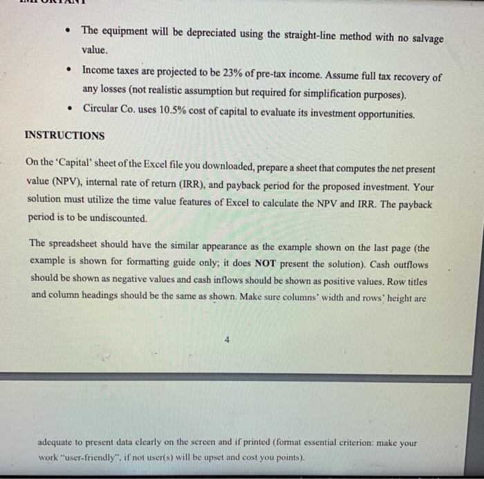
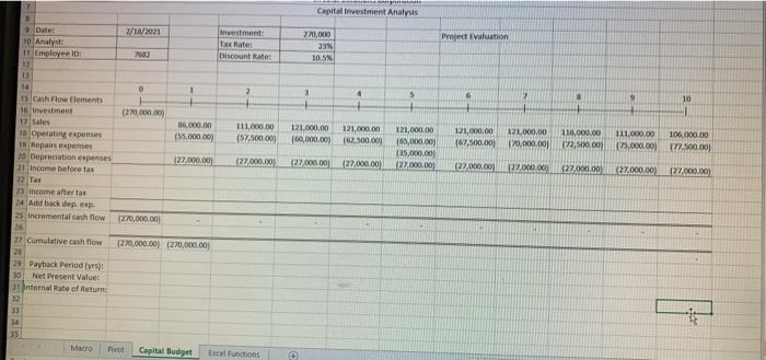
This exercise is comprised of four parts. Part 1 covers automated routines ‘macros’ in Excel to rearrange and transform data, Part 2 covers ‘Pivot’ Table: Data Sets Cross-Tabulation and Querying in Excel to extract and summarize data , Part 3 covers using Microsoft Excel spreadsheet software to construct, automate and analyze what-if-scenario for a sample budget/investment to help in decision making, and Part 4 has selected powerful Excel functions to assist in data analyses. Macros may not work on a Mac computer (relative reference feature in Macros was disabled in latest Excel for Mac!). Without this feature Macros will not work on a Mac computer. You can do the Macros Part 1 on a PC computer, then proceed working with the copy of restructured data using your Mac computer. Another advanced (complex) approach is to ‘virtually’ install Windows PC on your Mac (this is ‘on your own’ approach- not recommended and not supported by instructor). Please follow all display and formatting instructions for Part 3 (use WebEX class instructions too to save reading many formatting details in Part 3). Also, data set used every semester may change; the instructions below may reference range of cells for 12 months not 15 months; you adapt the months instructions based on the data set given/assigned on Blackboard (Bb). YOU ARE EXPECTED TO DO YOUR OWN WORK. Feel free, of course, to make use of the excellent help feature of Excel. If you work with other students, Do Not share your work with other students, or copy another student’s work into your Excel file/workbook. PART 1: CREATING AND EDITING A MACRO [5 POINTS] “To automate a repetitive task so that you can do the task again with a single click, you can record a macro in Excel.” (Microsoft Office documentation). Make sure you download or save the Excel file ’Excel_Macro_Data Analysis_Template_semesterYY.xlsm’ on Blackboard (Bb) to your hard-drive, then work off your workstation. • DO NOT invoke Excel by double-clicking or opening the file on Blackboard as this will allow you to open the Excel file on the internet utilizing most but maybe not all Excel 2 functionality and you may NOT have ownership of the file you work with and may not be able to save your work. Although this limitation is fading with new advanced ‘Cloud’ computing, it may still be an issue depending on the set-up of your PC and software). 1. Download the Excel file from Blackboard (filename: “Excel Macro_Data Analysis_Template_semesterYY.xlsm”) [click on file and select “Save” from the prompt screen or download then copy to desktop or USB depending on your browser]. 2. Then open the file using Excel on your desktop. 3. Sometimes your computer protects your files from viruses and open it in Protected View. To exit and start edit, click “Enable Editing” on the Message Bar. 4. Enter your name (in cell B3 of ‘Macro’ sheet) and student number (in cell B5 of ‘Macro’ sheet without the leading character “A”) before you start creating the macro. [make sure you do not delete any columns or rows in ‘Macro’ sheet or override format of cells B3 and B5] 5. Write a macro to move the data for the fields (columns) Date, Price, Shares, Account and Amount into five columns under the appropriate headings (i.e., the date data should begin in A21 and end around A386 and the price data should begin in B21 and end around B386 (or after/higher row# depending on data set given- maybe to cell B476, etc.). • When recording macros, make sure you are viewing the stop macro toolbar and set the recorder to record relative cell references. • Hints i. Use cut and paste commands and use end (up, down, right or left) commands where possible when constructing the macro. ii. Macros are used to automate repetitive actions and minimize manual spreadsheet keystrokes and activities. Your macro should not be more cumbersome than manual tasks and should not exceed more than ten lines of commands (class discussion-*01). *01- The macro should not have recordings of repetitive/duplicate individual cut and paste steps; this will create 5-6 pages of programming code involving doing the whole restructuring of the data manually with more than 64 cuts & pastes!!! NOT ACCEPTABLE and defeats the sole purpose of macros. 3 PART 2: PIVOT TABLE (EXCEL DATABASE FUNCTION) [10 POINTS] After ending with five columns of consecutive daily sales of shares, the data will be copied and used in Pivot worksheet (As an Internal Control DO NOT use the original data. Use the ‘Paste Options’ to paste the values in ‘Pivot’ sheet). Then, generate the following reports to help management perform trend analyses on summarized data: 1. Report 1: a report that totals the ‘Amount’ of sales by ACCOUNT across Months. 2. Report 2: summarizing the total amount of sales by Industry type of shares sold across Months [report should be categorized by industry number, ignore description of industry type – see data dictionary item (ii) below]. 3. Report 3: produce a Line chart to show the total monthly sales trend for the period given (place chart below the two pivot tables). Write two sentences analyzing/describing what the chart represents and the summary conclusion(s) revealed by the line chart. 4. HINTS: a. Use ‘Pivot Table’ in Excel (place the Pivot Tables on the right of the data in same ‘Pivot’ worksheet). b. Data Dictionary for Excel Downloaded Data. Account field or attribute is an alphanumeric field which is 7 digits or characters long. The field is composed of the following: • Digits 1-3, indicate ‘Revenue-Sales’ account (400-General Ledger Chart of Accounts). • Digits 4-5, indicate industry type of shares sold (Energy, International, Service, etc. type of funds). • Digits 6-7, indicate division or broker/custodian (financial institution) making the sale. PART 3: CAPITAL INVESTMENT ‘WHAT-IF’ ANALYSIS [25 POINTS] [Please see AUTOMATION AND MINIMAL MANUAL DATA ENTRY for Part 3 below] Circular Solutions Corporation is considering an expansion of their manufacturing capacity in order to produce a new golf ball to be introduced to the market. 4 • The equipment will cost $270,000 to purchase and install. • Incremental cash collections from sales are projected to be $86,000 for the first year, grow by $25,000 for the second year, and another $10,000 (compared to year 2) for years 3-7, decreasing thereafter by $5,000 each year through the remainder of the 10 years total life of the equipment as the popularity of the ball declines. • Incremental cash disbursements for product costs and operating expenses are projected to be $55,000 in the first year, increasing by $2,500 each year thereafter throughout the life of the project. • In addition, a major repair is expected to require one-time $35,000 cash expenditure (expense) at the end of the fifth year. • With the exception of the initial investment, which will occur at the beginning of the first year (i.e., at time 0), all cash flows can be assumed to occur at the end of the period. IMPORTANT • The equipment will be depreciated using the straight-line method with no salvage value. • Income taxes are projected to be 23% of pre-tax income. Assume full tax recovery of any losses (not realistic assumption but required for simplification purposes). • Circular Co. uses 10.5% cost of capital to evaluate its investment opportunities. INSTRUCTIONS On the ‘Capital’ sheet of the Excel file you downloaded, prepare a sheet that computes the net present value (NPV), internal rate of return (IRR), and payback period for the proposed investment. Your solution must utilize the time value features of Excel to calculate the NPV and IRR. The payback period is to be undiscounted. The spreadsheet should have the similar appearance as the example shown on the last page (the example is shown for formatting guide only; it does NOT present the solution). Cash outflows should be shown as negative values and cash inflows should be shown as positive values. Row titles and column headings should be the same as shown. Make sure columns’ width and rows’ height are 5 adequate to present data clearly on the screen and if printed (format essential criterion: make your work “user-friendly”, if not user(s) will be upset and cost you points). 1. Header: a. In the upper left: enter the date the exercise is submitted, your name as the analyst, and the last four digits of your student (A number) as the employee ID. b. In the upper center: i. Enter the initial investment (format as accounting, no $ sign, no decimals) ii. The tax rate (format as percentage with one decimal) iii. The discount rate (format as percentage with one decimal) in cells at the top left of the spreadsheet (see example). c. In the upper right: display the project evaluation as either: i. Net Value (NPV) > 0: “Accept Project” ii. Net Value (NPV) < 0: “Reject Project” iii. Net Value (NPV) = 0: “Indifferent” 2. Draw the horizontal time line by using the drawing capabilities of Excel. The vertical hash marks can be created by inserting the symbol using the insert and symbol menu selections. Enter the time period numbers in the cells above the hash marks. Be sure to center the hash marks and the numbers in their cells. 3. Formatting the cells: a. Format the data cells as accounting, no $ sign, with no decimals. b. Format the NPV output cell as accounting, no $ sign, with no decimals. c. Format the IRR output cell as percentage with two decimals. d. Format the undiscounted payback period output cell as number, with one decimal (i.e., assume that cash flow occurs evenly during, rather than at the end of, the payback year), and centered directly under the pointer. 4. Use IF statements containing an AND logical operator to display and position the pointer and the years to payback in the cells directly under the year in which payback occurs (see example below and as will be discussed in class). 6 a. If you are using Excel 2007 or a more recent version, you can insert the “▲” pointer symbol in a cell anywhere on the spreadsheet and reference the cell in the IF statement. b. Earlier versions of Excel may allow you to copy and insert symbol in the IF statement itself. c. As an alternative you can insert the “^” symbol directly from the keyboard by pressing shift_6 or for Excel 2010 you can insert the “▲” during creation of formula and in required spot by holding “Alt” and keying the number 30 (on numeric pad). d. The IF statement should be constructed such that the pointer and payback period are displayed only under the year in which payback occurs, with blank cells displaying under all other years. i. *The position of both should change if a change in parameters will increase or decrease the payback period forcing payback to occur during another year

 

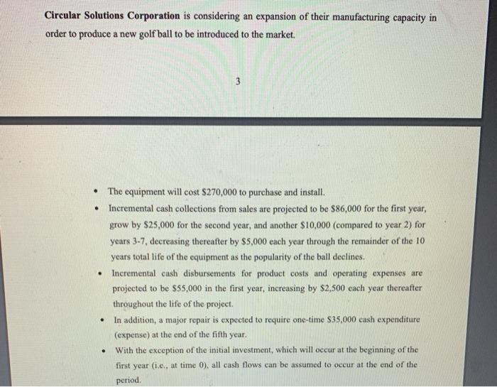
Circular Solutions Corporation is considering an expansion of their manufacturing capacity in order to produce a new golf ball to be introduced to the market. The equipment will cost $270,000 to purchase and install. Incremental cash collections from sales are projected to be $86,000 for the first year, grow by $25,000 for the second year, and another $10,000 (compared to year 2) for years 3-7, decreasing thereafter by $5,000 each year through the remainder of the 10 years total life of the equipment as the popularity of the ball declines. Incremental cash disbursements for product costs and operating expenses are projected to be $55,000 in the first year, increasing by $2,500 each year thereafter throughout the life of the project. In addition, a major repair is expected to require one-time $35,000 cash expenditure (expense) at the end of the fifth year. With the exception of the initial investment, which will occur at the beginning of the first year (i.c., at time 0), all cash flows can be assumed to occur at the end of the period. . . . 3