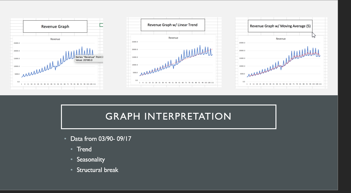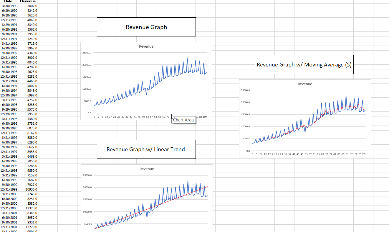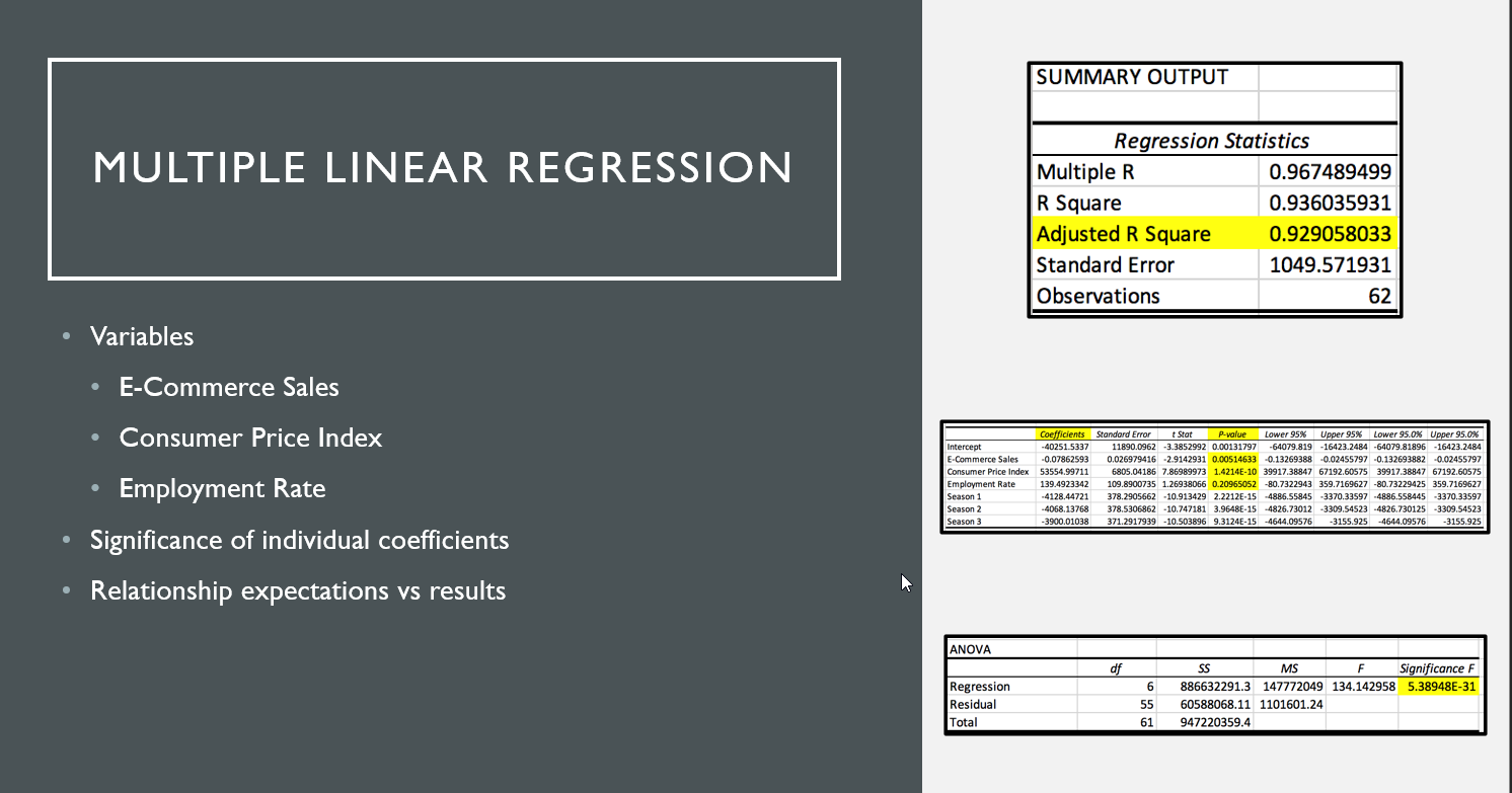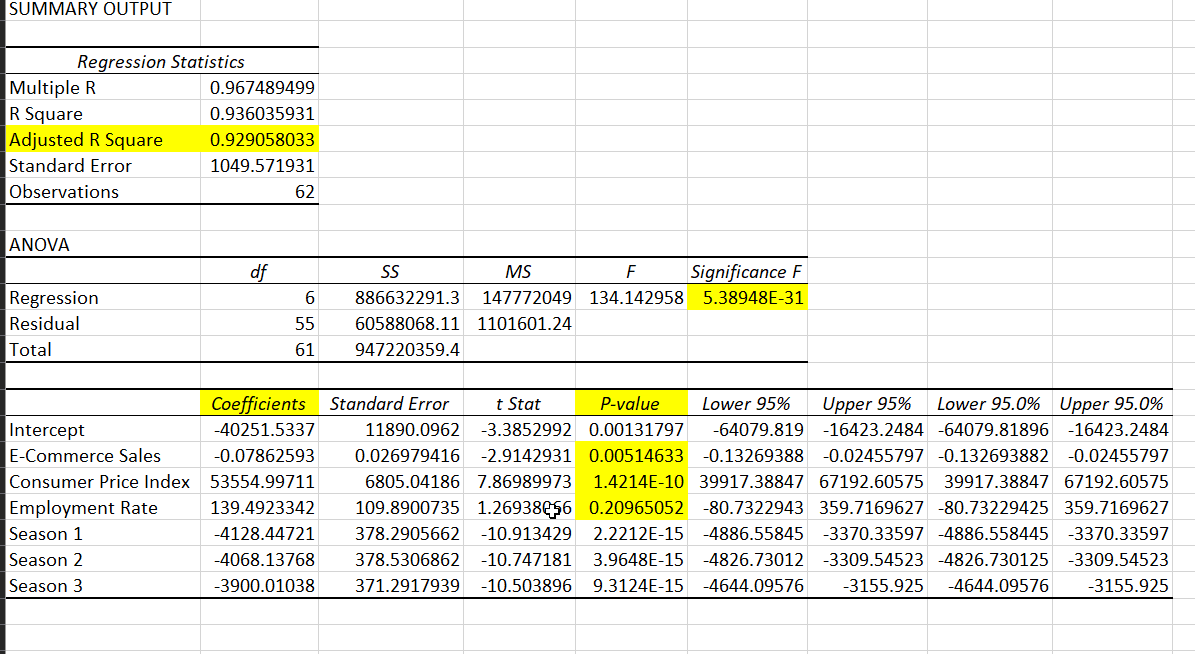
This has been solved. The missing part is the interpretation and the discussions as mentionned in Question 1, Question 2 & Question 2(ctd). Only the commentary/interpretation is needed. I have attached the slides and capture of the excel analysis as supporting documentation.

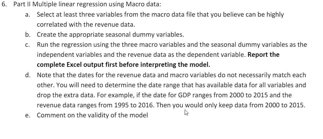
Part | Time Series analysis: discuss the revenue data similar to what I have showed in the Sears example is expected: scatter plot of revenue; linear trend; moving average; structural break. Your company revenue may not exhibit strong seasonality. For practice purpose; you are required to fit a moving average to your revenue data nevertheless. First explain what the graph tells you as a manager about the trend; seasonality, and structural break in this company data. Then conduct research to find out how management actually made the decisions in the data. f. Comment on the significance of individual coefficients. Briefly discuss the relationship (positive or negative} between the dependent variable and each of the independent variables with significant coefficient. Are those relationship expected? g. Report the adjusted r-squared and briefly comment on the fitness of the model based on your opinion. 6. Part II Multiple linear regression using Macro data: a. Select at least three variables from the macro data file that you believe can be highly correlated with the revenue data. Create the appropriate seasonal dummy variables. Run the regression using the three macro variables and the seasonal dummy variables as the independent variables and the revenue data as the dependent variable. Report the complete Excel output rst before interpreting the model. Note that the dates for the revenue data and macro variables do not necessarily match each other. You will need to determine the date range that has available data for all variables and drop the extra data. For example, if the date for GDP ranges from 2000 to 2015 and the revenue data ranges from 1995 to 2016. Then you would only keep data from 2000 to 2015. Comment on the validity of the model l} Revenue Graph C Revenue Graph w/ Linear Trend Revenue Graph w/ Moving Average (5) Revenue Revenue Revenue 20300 0 15000 Series "Revenue" Point 15300.0 Value: 20180.0 10060.a 1 6 13 36 21 26 38 36 41 46 51 36 63 06 71 76 81 86 91 96 160 306 101 GRAPH INTERPRETATION . Data from 03/90- 09/17 . Trend . Seasonality Structural breakSUMMARY OUTPUT Regression Statistics MULTIPLE LINEAR REGRESSION Multiple R 0.967489499 R Square 0.936035931 Adjusted R Square 0.929058033 Standard Error 1049.571931 Observations 62 Variables . E-Commerce Sales . Consumer Price Index Coefficients Standard Error t Stat P-value Lower 95% Upper 95% Lower 95.0% Upper 95.0% Intercept -40251.5337 11890.0962 -3.3852992 0.00131797 -64079.819 -16423.2484 -64079.81896 -16423.2484 E-Commerce Sales 0.07862593 0.026979416 -2.9142931 0.00514633 -0.13269388 -0.02455797 -0.132693882 -0.02455797 Consumer Price Index 53554.99711 6805.04186 7.86989973 1.4214E-10 39917.38847 67192.60575 39917.38847 67192.60575 Employment Rate Employment Rate 139.4923342 109.8900735 1.26938066 0.20965052 -80.7322943 359.7169627 -80.73229425 359.7169627 Season 1 -4128.44721 378.2905662 -10.913429 2.2212E-15 -4885.55845 -3370.33597 -4886.558445 -3370.33597 Season 2 -4068.13768 378.5306862 -10.747181 3.9648E-15 -4826.73012 -3309.54523 -4826.730125 -3309.54523 Season 3 -3900.01038 371.2917939 -10.503896 9.3124E-15 -4644.09576 -3155.925 -4644.09576 -3155.925 Significance of individual coefficients . Relationship expectations vs results ANOVA df SS MS Significance F Regression 6 886632291.3 147772049 134.142958 5.38948E-31 Residual 55 60588068.11 1101601.24 Total 61 947220359.4SUMMARY OUTPUT Regression Statistics Multiple R 0.967489499 R Square 0.936035931 Adjusted R Square 0.929058033 Standard Error 1049.571931 Observations 62 ANOVA df SS MS F Significance F Regression 6 886632291.3 147772049 134.142958 5.38948E-31 Residual 55 60588068.11 1101601.24 Total 61 947220359.4 Coefficients Standard Error t Stat P-value Lower 95% Upper 95% Lower 95.0% Upper 95.0% Intercept -40251.5337 11890.0962 -3.3852992 0.00131797 -64079.819 -16423.2484 -64079.81896 -16423.2484 E-Commerce Sales -0.07862593 0.026979416 -2.9142931 0.00514633 -0.13269388 -0.02455797 -0.132693882 -0.02455797 Consumer Price Index 53554.99711 6805.04186 7.86989973 1.4214E-10 39917.38847 67192.60575 39917.38847 67192.60575 Employment Rate 139.4923342 109.8900735 1.26938656 0.20965052 -80.7322943 359.7169627 -80.73229425 359.7169627 Season 1 -4128.44721 378.2905662 -10.913429 2.2212E-15 -4886.55845 -3370.33597 -4886.558445 -3370.33597 Season 2 -4068.13768 378.5306862 -10.747181 3.9648E-15 -4826.73012 -3309.54523 -4826.730125 -3309.54523 Season 3 -3900.01038 371.2917939 -10.503896 9.3124E-15 -4644.09576 -3155.925 -4644.09576 -3155.925Date Revenue 3/30/1990 3007.0 6/29/1990 3242.0 9/28/1990 3625.0 12/31/1990 4865.0 3/29/1991 3349.0 6/28/1991 3562.0 Revenue Graph 9/30/1991 3955.0 12/31/1991 5249.0 3/31/1992 3719.0 Revenue 6/30/1992 3967.0 9/30/1992 4340.0 25000.0 12/31/1992 5901.0 3/31/1993 4040.0 2000010 Revenue Graph w/ Moving Average (5) 6/30/1993 4287.0 9/30/1993 4625.0 12/31/1993 5281.0 15000.0 3/31/1994 4465.0 Revenue 6/30/1994 4802.0 10000.0 9/30/1994 5046.0 25000.0 12/30/1994 6998.0 3/31/1995 4757.0 500Q.0 20000.0 6/30/1995 5236.0 9/29/1995 5573.0 12/29/1995 7950.0 0.0 15000.0 1 5 9 13 17 21 25 29 33 37 41 45 49 53 57 61 65 69 73 101 106 109 3/31/1996 6380.0 Chart Area 6/30/1996 5751.0 10000.0 9/30/1996 6073.0 12/31/1996 8167.0 3/31/1997 5889.0 5000.0 6/30/1997 6293.0 9/30/1997 6622.0 Revenue Graph w/ Linear Trend 0.0 12/31/1997 8953.0 1 5 9 13 17 21 25 29 33 37 41 45 49 53 57 61 65 69 73 77 81 85 89 93 97 101106109 3/31/1998 6468.0 6/30/1998 7056.0 9/30/1998 7288.0 9850.0 Revenue 12/31/1998 3/31/1999 7158.0 25000.0 6/30/1999 7687.0 9/30/1999 7927.0 20000.0 12/31/1999 10930.0 3/31/2000 7746.0 6/30/2000 8251.0 15000.0 9/30/2000 3582.0 12/31/2000 12320.0 3/31/2001 8345.0 10000.0 6/30/2001 8952.0 9/30/2001 9331.0 500 0.0 12/31/2001 13220.0Date Revenue E-Commerce Sales Consumer Price Index Employment Rate Season 1 Season 2 Season 3 9/30/1999 7927.0 4448 0.7724 74.0 12/31/1999 10930.0 5816 0.7801 74.2 3/31/2000 7746.0 6501 0.7862 74.3 6/30/2000 8251.0 7333 0.7934 73.9 9/30/2000 8582.0 7766 0.7990 74.0 12/31/2000 12320.0 8220 0.8067 73.9 3/31/2001 8345.0 8357 0.8123 73.4 O O H O O O H O O O H O O O O H O O O H O O O H O O O P O O O H O O O H O O O P O O 6/30/2001 8952.0 8276 0.8146 72.8 9/30/2001 9331.0 9307 0.8140 72.3 12/31/2001 13220.0 10000 0.8166 72.2 3/31/2002 9594.0 10756 0.8230 71.9 6/30/2002 10070.0 11478 0.8275 71.9 9/30/2002 10190.0 12227 0.8324 71.7 12/31/2007 7554 0 12796 0 8409 715