This is a .ipynb file, please fill out the function of basket_option based on the instruction (this is not a big project, just basic stuff):

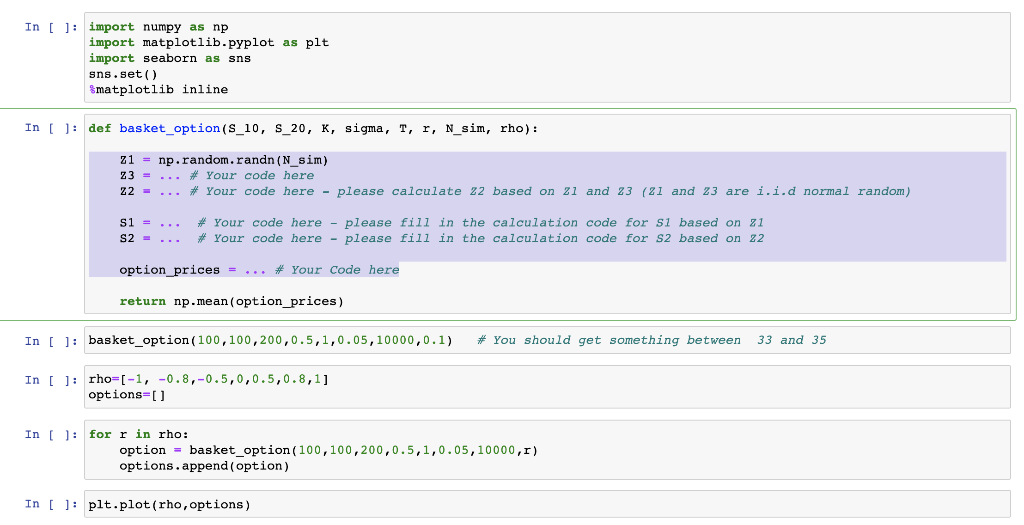
Code for copy:

import numpy as np import matplotlib.pyplot as plt import seaborn as sns sns.set() %matplotlib inline

def basket_option(S_10, S_20, K, sigma, T, r, N_sim, rho): Z1 = np.random.randn(N_sim) Z3 = ... # Your code here Z2 = ... # Your code here - please calculate Z2 based on Z1 and Z3 (Z1 and Z3 are i.i.d normal random) S1 = ... # Your code here - please fill in the calculation code for S1 based on Z1 S2 = ... # Your code here - please fill in the calculation code for S2 based on Z2 option_prices = ... # Your Code here return np.mean(option_prices)

basket_option(100,100,200,0.5,1,0.05,10000,0.1) # You should get something between 33 and 35

rho=[-1, -0.8,-0.5,0,0.5,0.8,1] options=[]

for r in rho: option = basket_option(100,100,200,0.5,1,0.05,10000,r) options.append(option)

plt.plot(rho,options)

European Basket Option Price Use Monte Carlo simulation to calculate a European basket option price where the payoff at expiry T is defined as Payoff (T) = max(S1(T) + S2(T) K,0) The two Stock prices S and S2 follows correlated Geometric Brownian Motion: Si(T) = Si(0) exp((r 102)T +oBr) S2(T) = S2(0) exp((r 202)T +oWT) Where By = VTZ, W1 = VTZ2, Z, ~ N(0,1), Z2 ~ N(0,1) corr(Z1, Z2) = Here . Si(0) = S2(0) = 100 K = 200 0 = 0.5 T = 1 r = 0.05 Remember option price is the average discounted payoff: C = E[e-rT max(Si(T) + S2(T) K,O] calculate and plot the option prices for p = -1,-0.8,-0.5,0,0.5, 0.8, 1, and plot C as p changes In [ ]: import numpy as np import matplotlib.pyplot as plt import seaborn as sns sns.set() Smatplotlib inline In [ ]: def basket_option(S_10, S_20, K, sigma, T, r, N_sim, rho): z1 = np.random.randn (N_sim) Z3 = ... # Your code here Z2 = # Your code here - please calculate 22 based on 21 and 23 (21 and 23 are i.i.d normal random) S1 = S2 = ... # Your code here - please fill in the calculation code for si based on 21 # Your code here - please fill in the calculation code for s2 based on 22 option_prices = ... * Your Code here return np.mean(option_prices) In [ ]: basket_option (100,100,200,0.5,1,0.05,10000,0.1) # You should get something between 33 and 35 In [ ]: rho=(-1, -0.8,-0.5,0,0.5,0.8,1] options=[] In [ ]: for r in rho: option = basket_option (100,100,200,0.5,1,0.05,10000,1) options.append(option) In [ ]: plt.plot(rho, options) European Basket Option Price Use Monte Carlo simulation to calculate a European basket option price where the payoff at expiry T is defined as Payoff (T) = max(S1(T) + S2(T) K,0) The two Stock prices S and S2 follows correlated Geometric Brownian Motion: Si(T) = Si(0) exp((r 102)T +oBr) S2(T) = S2(0) exp((r 202)T +oWT) Where By = VTZ, W1 = VTZ2, Z, ~ N(0,1), Z2 ~ N(0,1) corr(Z1, Z2) = Here . Si(0) = S2(0) = 100 K = 200 0 = 0.5 T = 1 r = 0.05 Remember option price is the average discounted payoff: C = E[e-rT max(Si(T) + S2(T) K,O] calculate and plot the option prices for p = -1,-0.8,-0.5,0,0.5, 0.8, 1, and plot C as p changes In [ ]: import numpy as np import matplotlib.pyplot as plt import seaborn as sns sns.set() Smatplotlib inline In [ ]: def basket_option(S_10, S_20, K, sigma, T, r, N_sim, rho): z1 = np.random.randn (N_sim) Z3 = ... # Your code here Z2 = # Your code here - please calculate 22 based on 21 and 23 (21 and 23 are i.i.d normal random) S1 = S2 = ... # Your code here - please fill in the calculation code for si based on 21 # Your code here - please fill in the calculation code for s2 based on 22 option_prices = ... * Your Code here return np.mean(option_prices) In [ ]: basket_option (100,100,200,0.5,1,0.05,10000,0.1) # You should get something between 33 and 35 In [ ]: rho=(-1, -0.8,-0.5,0,0.5,0.8,1] options=[] In [ ]: for r in rho: option = basket_option (100,100,200,0.5,1,0.05,10000,1) options.append(option) In [ ]: plt.plot(rho, options)