THIS IS THE LINK https://ophysics.com/k7.html , PLEASE DO THIS ACTIVITY ON A COMPUTER GO TO THE WEBSITE LINK THAT I PUT THE SAME LINK UNDER MATERIALS PLEASE COPY THE LINK ON YOUR COMPUTER TO DO THE EXCERSICES, THANK YOU.

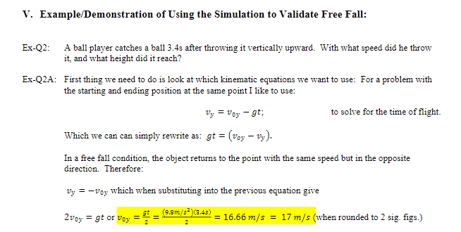
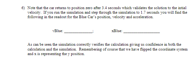
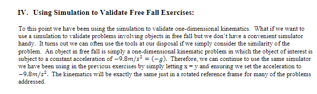
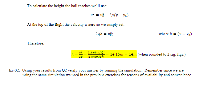
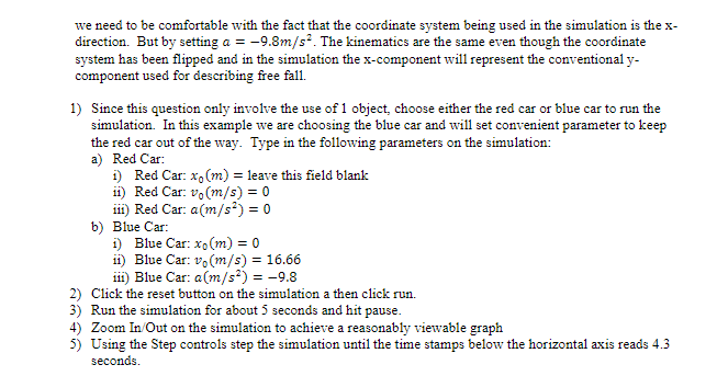
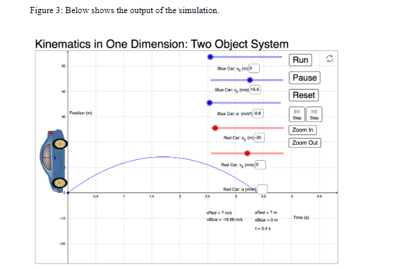
Objective: In this labfsimulation we will look at the power of simulations to validate calculations anda'or the needs to often perform estimates, in these cases a simulation is given some initial conditions. In physics, as well as other sciences and engineering we often develop simulations to solve problems that do not readily have closed form mathematical solutions. This us allows one to simulate the response of designs of instrmnents and mechanisms to external forces and stimuli such as vibration, shock, thermal changes, movement of objects through various medium (Le. drag), etc. For example, the drag, a car experiences when travelling at speed due to air resistance, or the resistance a boat experiences moving through water. Other examples might include the resistance of blood owing through arteries and veins as a diagnostic for medical conditions. One of the key confidence tests for a simulation is to test the simulations results against known solutions. In addition, to using these lmown conditions to test the validity of a simulator the simulator is oen used to validate calculations, especially those involving complex calculations. In this labr'sirnulation, we will solve several questions, and then input the results of the calculation to validate the calculated solution. We will also explore using a simulation designed for a particular set of conditions and adapting it for other situations by simply adjusting the initial conditions andx'or looking at the results at various time steps while interpreting the result between the time steps. Materials: This handout Attendance of the mini-lecture lab introduction kinematics in one dimension along with the demonstration of the simulation . Computer and Internet access to use the following simulation: https://ophysics.com/k7.html I. Starting and Exploring the Simulation: Note: The figures shown below as well as the some of the controls may vary depending on the internet browser and hardware you are using. The figures and description below were generated by running the simulation by using: Internet Browser: Google Chrome Version 97.0.4692.99 Hardware: Apple macbook pro Operating System: macOS Montery Version 12.0.1 Your hardware software do not need to be the same but there may be subtle differences in the response of the controls. Purpose: To familiarize yourselves with the simulation along with the various windows and controls.IV. Using Simulation to Validate Free Fall Exercises: To this point we have been using the simulation to validate one-dimensional kinematics. What if we want to use a simulation to validate problems involving objects in free fall brutwe don't have a convenient simulator handy. It turns out we can often use the tools at our disposal ifwe simply consider the similarity ofthe problem. An object in free fall is simply a one-dimensional kinematic problem in which the object of interest is subject to a constant acceleration of '.':l.l3~:'1n.,l".sS = (9). Therefore, we can continue to use the same simulator we have been using in the prmious exercises by simply letting a = y and ensuring we set the acceleration to 9.Smf.s:. The kinematics will be exactly the same just in a rotated reference frame for many of the problems addressed V. Example/Demonstration of Using the Simulation to Validate Free Fall: Ex-Q2: A ball player catches a ball 3.4s after throwing it vertically upward. With what speed did he throw it, and what height did it reach? Ex-Q2A: First thing we need to do is look at which kinematic equations we want to use: For a problem with the starting and ending position at the same point I like to use: Vy = Voy - 9t: to solve for the time of flight. Which we can can simply rewrite as: gt = (voy - vy ). In a free fall condition, the object returns to the point with the same speed but in the opposite direction. Therefore: vy = -voy which when substituting into the previous equation give (9.8m/=>)(2.43) 2voy = gt of Voy = gt = 16.66 m/s = 17 m/s (when rounded to 2 sig. figs.)To calculate the height the ball reaches we'll use: v2 = 13 - 2g(1 - yo) At the top of the flight the velocity is zero so we simply set: 2gh = v6; where h = (x - xo) Therefore: h= - (16.66m/3)- = 14.16m = 14m (when rounded to 2 sig. figs.) 29 2.(9 8m/8-) Ex-$2: Using your results from Q2 verify your answer by running the simulation: Remember since we are using the same simulation we used in the previous exercises for reasons of availability and conveniencewe need to be comfortable with the fact that the coordinate system being used in the simulation is the x- direction. But by setting a = -9.8m/s'. The kinematics are the same even though the coordinate system has been flipped and in the simulation the x-component will represent the conventional y- component used for describing free fall. 1) Since this question only involve the use of 1 object, choose either the red car or blue car to run the simulation. In this example we are choosing the blue car and will set convenient parameter to keep the red car out of the way. Type in the following parameters on the simulation: a) Red Car: i) Red Car: Xo (m) = leave this field blank ii) Red Car: vo (m/s) = 0 iii) Red Car: a(m/s) = 0 b) Blue Car: i) Blue Car: xo(m) = 0 fi) Blue Car: Vo (m/s) = 16.66 iii) Blue Car: a (m/s ) = -9.8 2) Click the reset button on the simulation a then click run. 3) Run the simulation for about 5 seconds and hit pause. 4) Zoom In/Out on the simulation to achieve a reasonably viewable graph 5) Using the Step controls step the simulation until the time stamps below the horizontal axis reads 4.3 seconds.Figure 3: Below shows the output of the simulation. Kinematics in One Dimension: Two Object System Run C Pause Blue Car Y Imis) 16.6 Reset Puation /ml Blue Car. a imbi 90 Zoom In Red Car * (mi -30 Zoom Out Red Car: " (mb) 0 And Cara (miby Time (8)6) Note that the car returns to position zero after 3.4 seconds which validates the solution to the intial velocity. If you run the simulation and step through the simulation to 1.7 seconds you will find the following in the readout for the Blue Car's position, velocity and acceleration. vBlue: xBlue: As can be seen the simulation correctly verifies the calculation giving us confidence in both the calculation and the simulation. Remembering of course that we have flipped the coordinate system and x is representing the y position