This question will be utilizing python

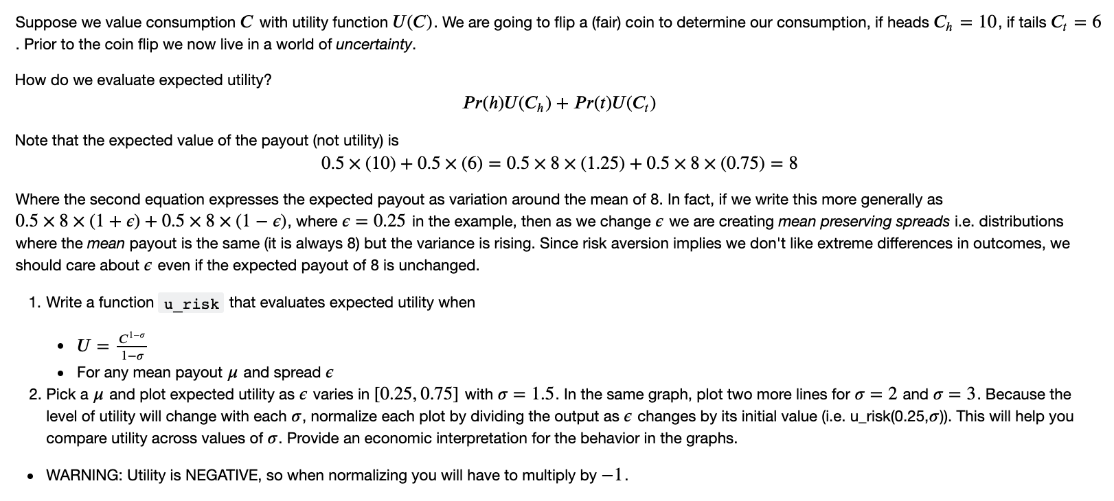
10, if tails C 6 Suppose we value consumption C with utility function U(C). We are going to flip a (fair) coin to determine our consumption, if heads Ch . Prior to the coin flip we now live in a world of uncertainty. How do we evaluate expected utility? Pr(h)U(Ch) + Pr(t)U(C) Note that the expected value of the payout (not utility) is 0.5 X (10) + 0.5 x (6) = 0.5 X 8 X (1.25) +0.5 X 8 X (0.75) = 8 Where the second equation expresses the expected payout as variation around the mean of 8. In fact, if we write this more generally as 0.5 X 8 X(1 + ) + 0.5 X 8 X(1 e), where e = 0.25 in the example, then as we change e we are creating mean preserving spreads i.e. distributions where the mean payout is the same (it is always 8) but the variance is rising. Since risk aversion implies we don't like extreme differences in outcomes, we should care about e even if the expected payout of 8 is unchanged. 1. Write a function u_risk that evaluates expected utility when cl-o U = 1- For any mean payout u and spread e 2. Pick a u and plot expected utility as e varies in [0.25, 0.75] with o = 1.5. In the same graph, plot two more lines for o = 2 and o = 3. Because the level of utility will change with each o, normalize each plot by dividing the output as e changes by its initial value (i.e. u_risk(0.25,0)). This will help you compare utility across values of o. Provide an economic interpretation for the behavior in the graphs. WARNING: Utility is NEGATIVE, so when normalizing you will have to multiply by -1. 10, if tails C 6 Suppose we value consumption C with utility function U(C). We are going to flip a (fair) coin to determine our consumption, if heads Ch . Prior to the coin flip we now live in a world of uncertainty. How do we evaluate expected utility? Pr(h)U(Ch) + Pr(t)U(C) Note that the expected value of the payout (not utility) is 0.5 X (10) + 0.5 x (6) = 0.5 X 8 X (1.25) +0.5 X 8 X (0.75) = 8 Where the second equation expresses the expected payout as variation around the mean of 8. In fact, if we write this more generally as 0.5 X 8 X(1 + ) + 0.5 X 8 X(1 e), where e = 0.25 in the example, then as we change e we are creating mean preserving spreads i.e. distributions where the mean payout is the same (it is always 8) but the variance is rising. Since risk aversion implies we don't like extreme differences in outcomes, we should care about e even if the expected payout of 8 is unchanged. 1. Write a function u_risk that evaluates expected utility when cl-o U = 1- For any mean payout u and spread e 2. Pick a u and plot expected utility as e varies in [0.25, 0.75] with o = 1.5. In the same graph, plot two more lines for o = 2 and o = 3. Because the level of utility will change with each o, normalize each plot by dividing the output as e changes by its initial value (i.e. u_risk(0.25,0)). This will help you compare utility across values of o. Provide an economic interpretation for the behavior in the graphs. WARNING: Utility is NEGATIVE, so when normalizing you will have to multiply by -1