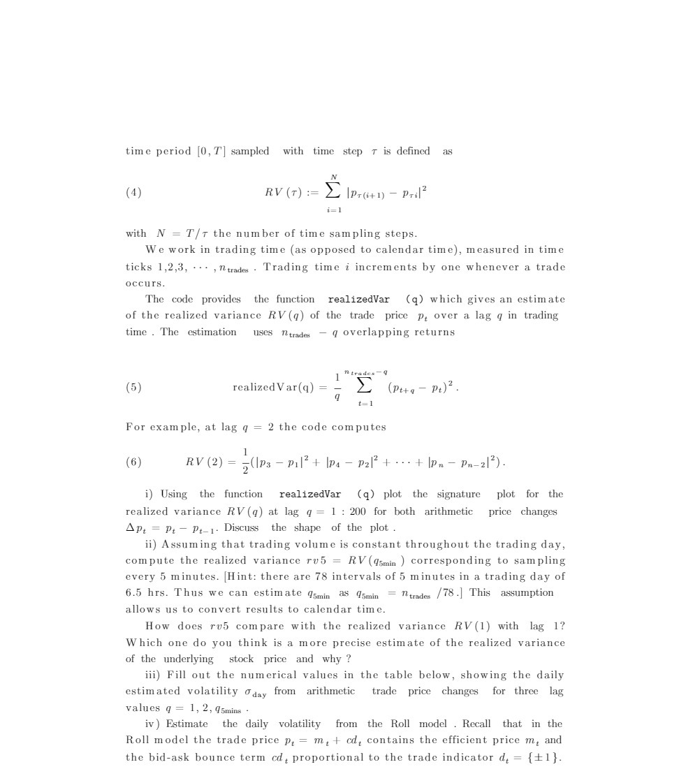
time period [0,T] sampled with time step T is dened as N (a) mm := Z lat-+1, Jun-F i=1 with N = TIT the number of time sampling steps' We work in trading time {as opposed to calendar time), measured in time ticks 1,2,3, . - . ,num . Trading time i increments by one whenever a trade occurs. The code provides the function I'ealized'i'ar ((1) which gives an estimate of the realized variance RV[q) of the trade price Fr over a lag q in trading time . The cstimation uses sum q overlapping returns \"(ruin'1 Z (50\".; Fe): - t=1 l (5) TDaliZedVar(q) = _ '5' For example, at lag q = 2 the cede computes 1 {5} RV(2} _ 2UP; Filzl L\": 192': l + an pn_2|2)_ i] Using the Function Iealized'lar (q) plot the signature plot for the realized variance RV{q) at lag q = 1 : 2{J(| for both arithmetic price changes th 2 Fr pk]. Discuss the shape of the plot . ii) Assuming that trading volume is constant throughout the trading day, compute the realized variance r125 = RV{q5min } corresponding to sampling every 5 minutes. [Hint: there are 78 intervals of 5 minutes in a trading day of 6.5 hrs. Thus we can estimate am as qmin = \"um JW3] This assumption allows 11s to convert results to calendar time. Hov.r does r05 compare with the realized variance RV(1) with lag 1? Which one do you think is a more precise estimate of the realized variance of the underlying stock price and why,r '? iii) Fill out the numerical values in the table below, showing the daily estimated volatility ads! from arithmetic trade price changes for three lag values q =1,'2,q5m1 iv] Estimate the daily volatility from the Roll mode] . Recall that in the Hell model the trade price p]! 2 mt + aft contains the efficient price sli.I and the hidask bounce term ad, proportional to the trade indicator d3 = {:l: l }