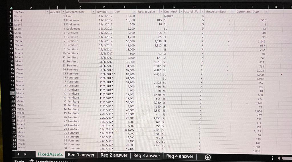
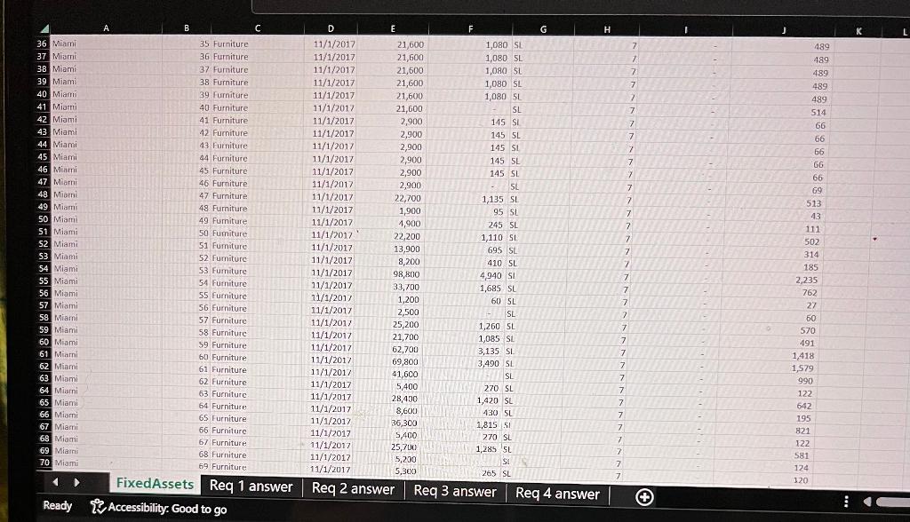
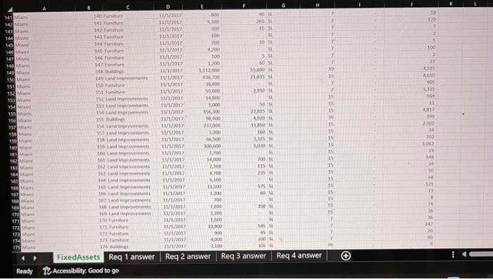
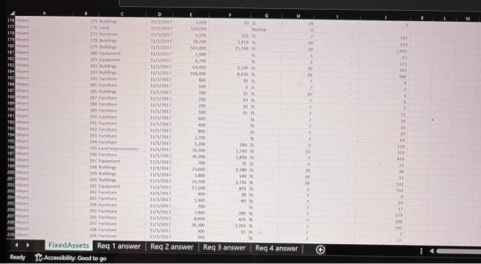
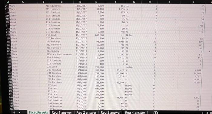
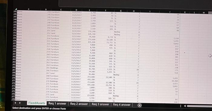
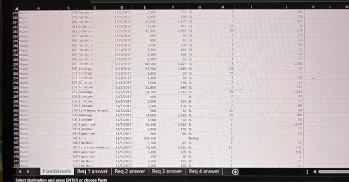
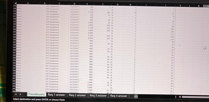
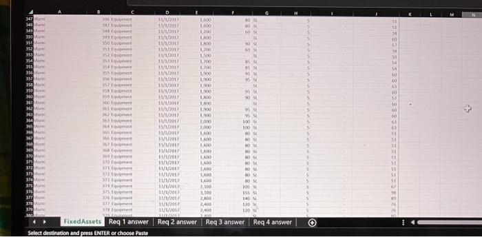
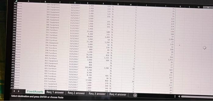
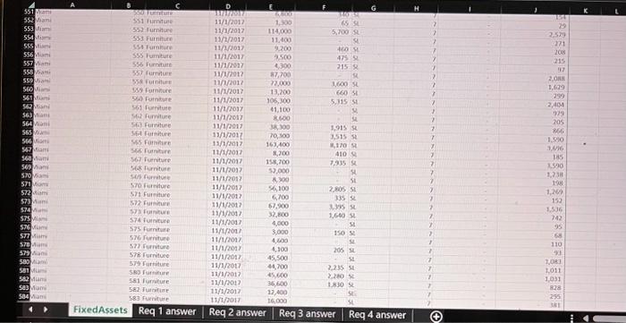
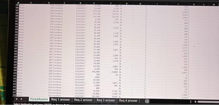
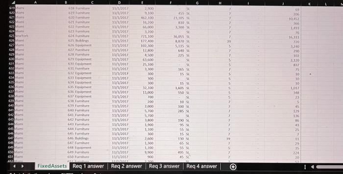
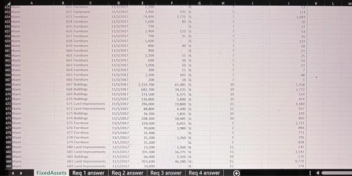
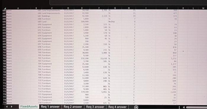
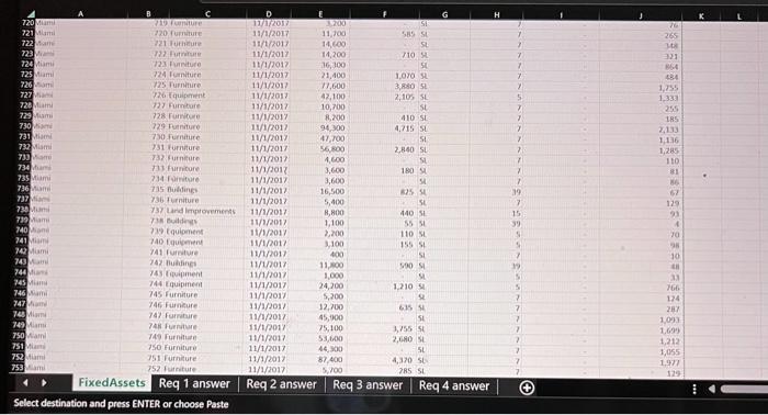
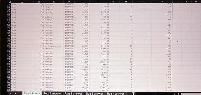
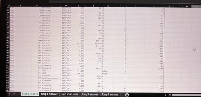
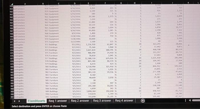
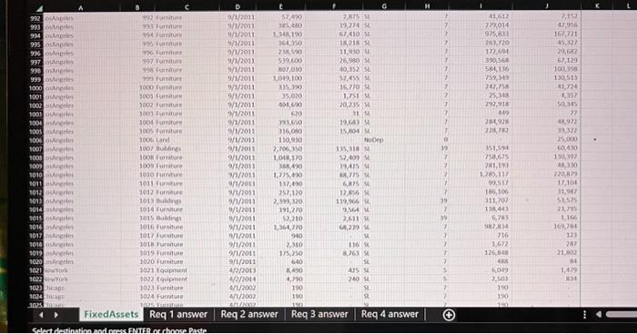
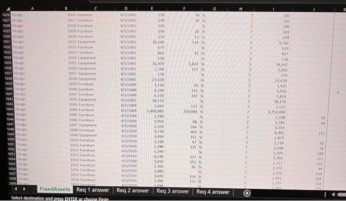
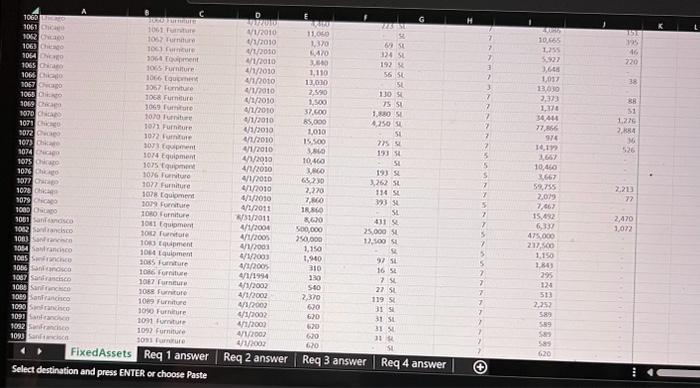
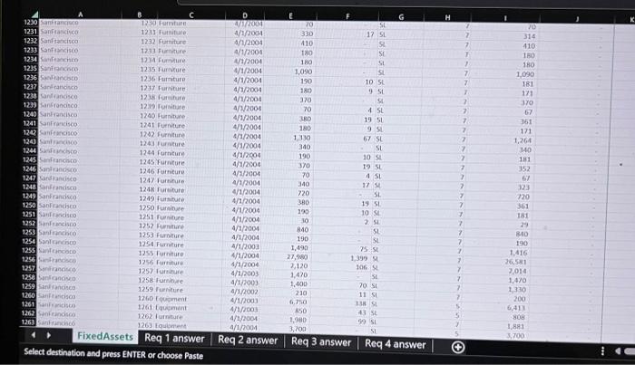
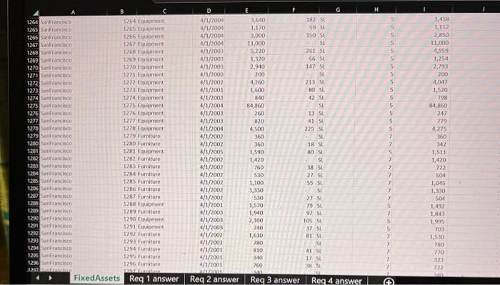
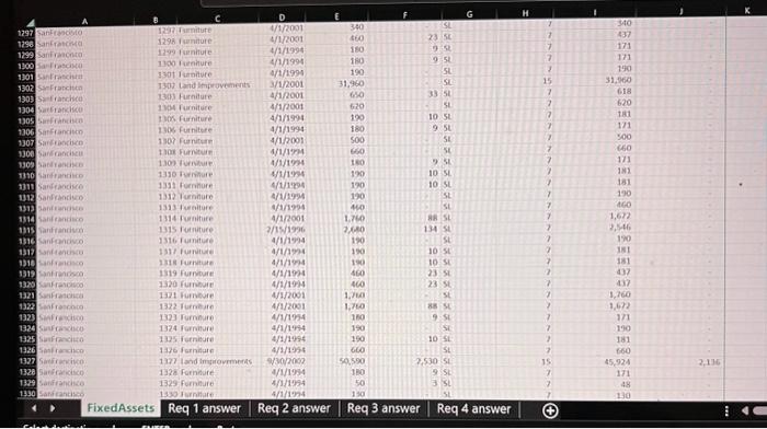
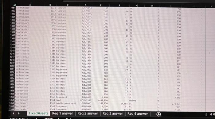
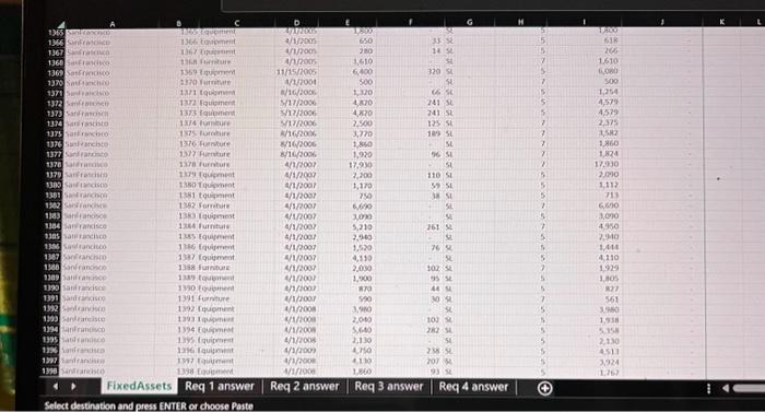
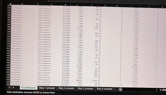
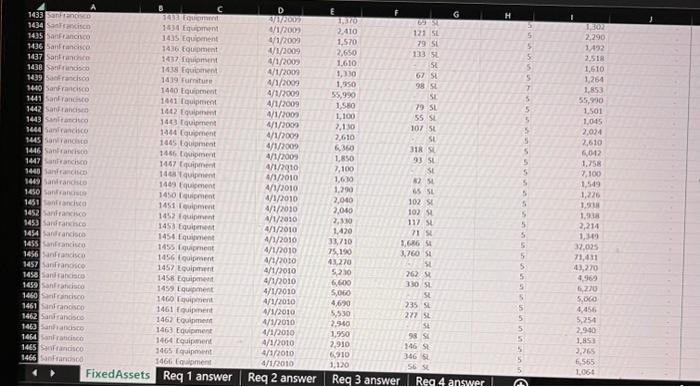
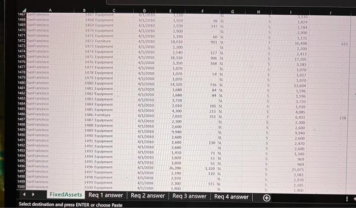
Tonis Tacos Learning objectives 1. Create a pivot table in Excel 2. Format a pivot table 3. Apply filters to a pivot table 4. Create sum columns in a pivot table 5. Create a calculated field 6. Use the slicer tool in a pivot table 7. Analyze data for errors 8. Create a pivot chart in Excel Data set background Toni Tapler, owner of Tonis Tacos has contacted your accounting firm to review her fixed asset records. Tonis Tacos specializes in serving authentic Mexican food. The company divides its reporting into six different city areas where the restaurants are located. These city areas are Boston, Chicago, Los Angeles, Miami, New York, and San Francisco. Toni has provided you with a spreadsheet containing the companys fixed asset data and has asked that your firm prepare a fixed asset schedule and answer various questions concerning the companys fixed assets. In addition to the fixed asset data, Toni included the following information from the companys fixed asset policies and procedures manual. Fixed asset categories are defined as follows: Land Vacant land parcels purchased for building sites, parking lots, or other purposes. Land Improvements Site improvements (other than buildings) such as fencing and parking lots. Buildings Permanent structures (including permanently attached fixtures). Equipment Self-explanatory. Furniture Self-explanatory. Data dictionary CityArea: Indicates the city area location of the fixed asset. AssetID: This field is a sequential number assigned at purchase. This is a unique identified. AssetCategory: Indicates the fixed asset category. InSvcDate: This is the date the asset was put into service. Cost: The purchase price of the asset. SalvageValue: The salvage value assigned by the company. DeprMeth: The depreciation method used for the asset. NoDep indicates that no depreciation is being calculated. SL indicates the asset is being depreciated using the straight-line convention. Useful Life: The useful life assigned by the company. BegAccumDepr: Beginning accumulated depreciation as of 1/1/2017. CurrentYearDepr: Current year depreciation for 2017. Requirements: For each of the following requirements, create a new pivot table in a new worksheet in Excel. Name each new worksheet as Req 1, Req 2, etc. Format the dollar amounts in each pivot table or pivot chart using the accounting format with zero decimal places. Format non-currency numbers in each pivot table or pivot chart using the accounting format with zero decimal places. Place your name in cell A1 of the worksheets. Review assignment rubric for specific grade evaluation 1. Prepare a pivot table of a fixed asset schedule that contains the totals for cost, beginning accumulated depreciation, current year depreciation, ending accumulated depreciation, and ending book value by city. (Hint: Create a calculated field for Ending Accumulated Depreciation and Ending Book Value.) What is the total ending book value for the Los Angeles area? How much depreciation was taken during the year for the entire company? 2. Which city(s) does not have land? 3. There is a concerned that there might be some errors in the data for the Los Angeles area. Prepare a fixed asset schedule (similar to requirement 1) for the Los Angeles area by asset category. Identify the asset ID which has the error and explain the error involved. (Hint: Use the slicer. Dont worry about checking any calculations.) 4. Prepare a pivot table that shows the book value of the furniture category by city area. Prepare a pivot chart using the column chart type for this information.

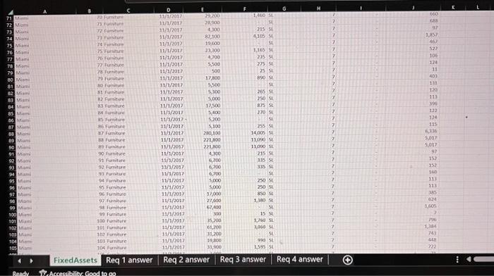
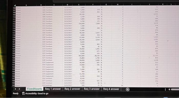
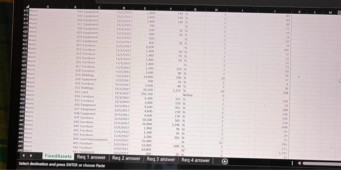
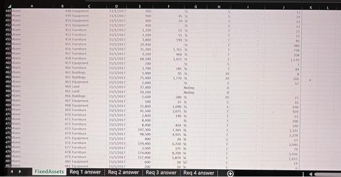
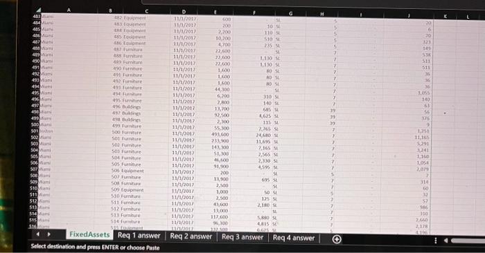
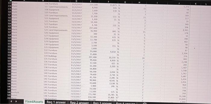
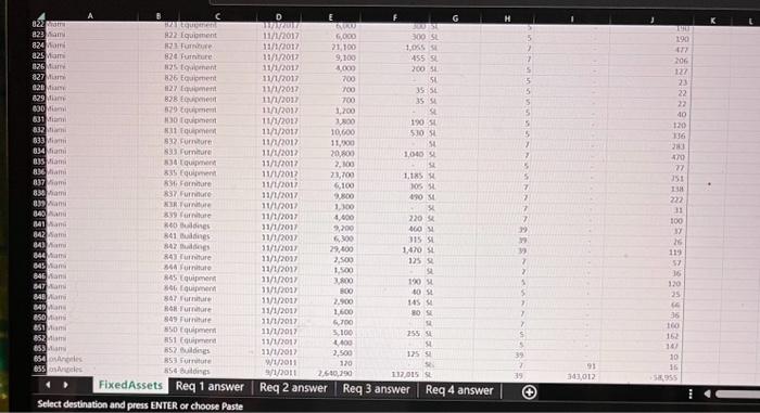
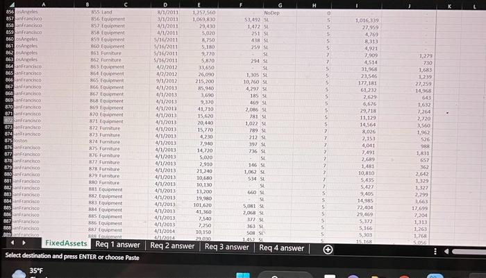
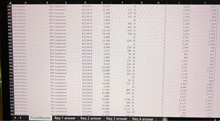
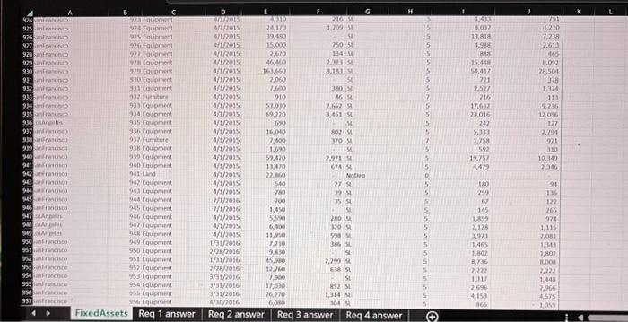
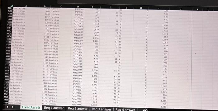
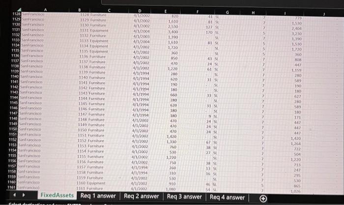
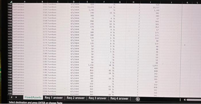
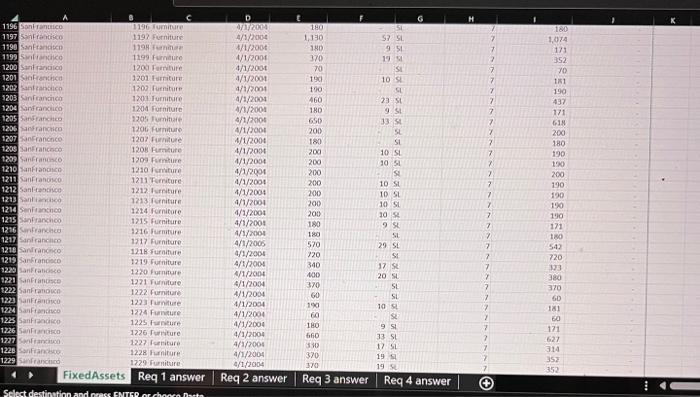
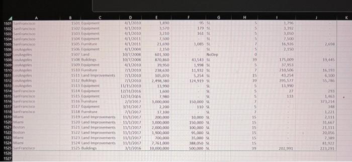
The excel sheet goes down 1,525 rows

(f) F \begin{tabular}{l} x7 \\ 82 \\ 32 \\ 33 \\ \hline \end{tabular} x.30=i (5) P 4 (4) 8