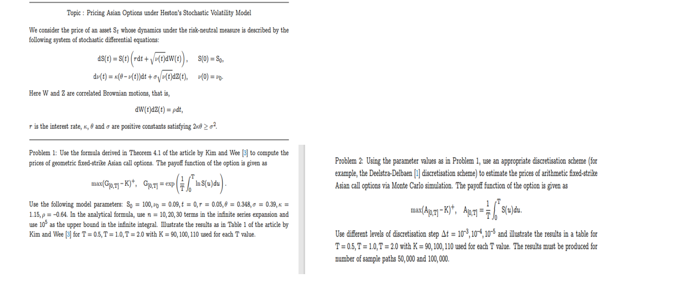
Topic : Pricing Asian Options under Heston's Stochastic Volatility Model We consider the price of an asset St whose dynamics under the risk-neutral measure is described by the following system of stochastic differential equations: ds(t) = s(e) (rat + Vu(t)aw(e)), S(O) = , M dy(t) = x(0-v(t))dt +Vu(t)dz(t), v(0) = vo. Here W and Z are correlated Brownian motions, that is, dW(t)dz(t) = pdt, r is the interest rate, 4, 6 and o are positive constants satisfying 2x0 > o? Problem 1: Use the formula derived in Theorem 4.1 of the article by Kim and Wee [3] to compute the prices of geometric fixed-strike Asian call options. The payoff function of the option is given as max(Gjo,r1 K)*, Go,r1 = exp PES In S(u)du ). Problem 2: Using the parameter values as in Problem 1, use an appropriate discretisation scheme (for example, the Deelstra-Delbaen (1) discretisation scheme) to estimate the prices of arithmetic fixed-strike Asian call options via Monte Carlo simulation. The payoff function of the option is given as 1 Use the following model parameters: So = 100,00 = 0.09, t = 0, = 0.05,0 = 0.348,0 = 0.39, K = 1.15, p = -0.64. In the analytical formula, use n = 10,20,30 terms in the infinite series expansion and use 106 as the upper bound in the infinite integral. Illustrate the results as in Table 1 of the article by Kim and Wee (3) for T = 0.5, T = 1.0, T = 2.0 with K = 90, 100, 110 used for each T value. mat(qon - *, Apon = [*sledu Use different levels of discretisation step At = 10-3,104,10-5 and illustrate the results in a table for T = 0.5, T = 1.0, T = 2.0 with K = 90,100,110 used for each T value. The results must be produced for number of sample paths 50,000 and 100,000. Topic : Pricing Asian Options under Heston's Stochastic Volatility Model We consider the price of an asset St whose dynamics under the risk-neutral measure is described by the following system of stochastic differential equations: ds(t) = s(e) (rat + Vu(t)aw(e)), S(O) = , M dy(t) = x(0-v(t))dt +Vu(t)dz(t), v(0) = vo. Here W and Z are correlated Brownian motions, that is, dW(t)dz(t) = pdt, r is the interest rate, 4, 6 and o are positive constants satisfying 2x0 > o? Problem 1: Use the formula derived in Theorem 4.1 of the article by Kim and Wee [3] to compute the prices of geometric fixed-strike Asian call options. The payoff function of the option is given as max(Gjo,r1 K)*, Go,r1 = exp PES In S(u)du ). Problem 2: Using the parameter values as in Problem 1, use an appropriate discretisation scheme (for example, the Deelstra-Delbaen (1) discretisation scheme) to estimate the prices of arithmetic fixed-strike Asian call options via Monte Carlo simulation. The payoff function of the option is given as 1 Use the following model parameters: So = 100,00 = 0.09, t = 0, = 0.05,0 = 0.348,0 = 0.39, K = 1.15, p = -0.64. In the analytical formula, use n = 10,20,30 terms in the infinite series expansion and use 106 as the upper bound in the infinite integral. Illustrate the results as in Table 1 of the article by Kim and Wee (3) for T = 0.5, T = 1.0, T = 2.0 with K = 90, 100, 110 used for each T value. mat(qon - *, Apon = [*sledu Use different levels of discretisation step At = 10-3,104,10-5 and illustrate the results in a table for T = 0.5, T = 1.0, T = 2.0 with K = 90,100,110 used for each T value. The results must be produced for number of sample paths 50,000 and 100,000


