Tutor please address this

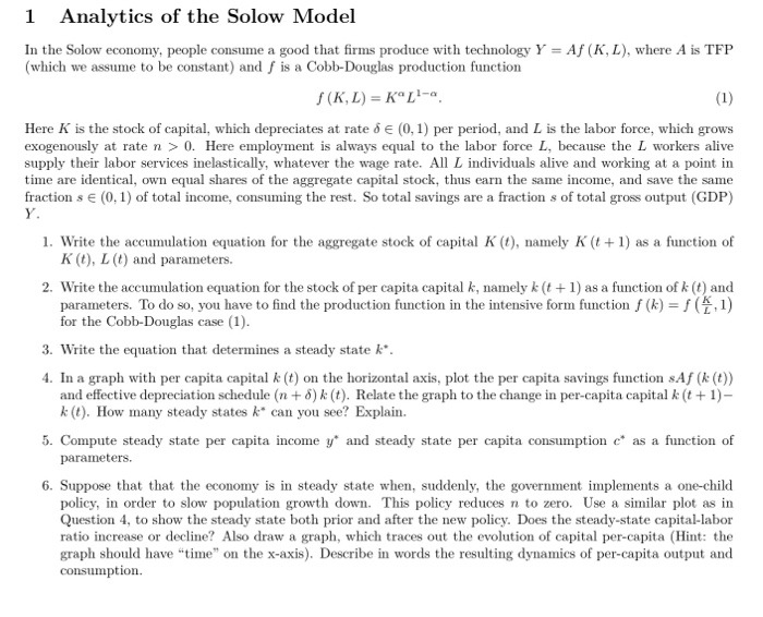
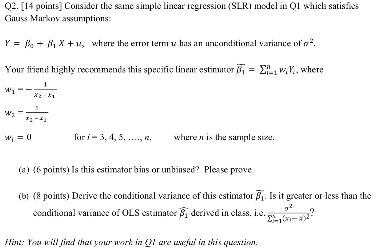
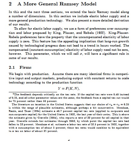
1 Analytics of the Solow Model In the Solow economy, people consume a good that firms produce with technology Y = Af (K, L), where A is TFP (which we assume to be constant) and f is a Cobb-Douglas production function f ( K, L) = KOL-a. (1) Here K is the stock of capital, which depreciates at rate o e (0, 1) per period, and L is the labor force, which grows exogenously at rate n > 0. Here employment is always equal to the labor force L, because the L workers alive supply their labor services inelastically, whatever the wage rate. All L individuals alive and working at a point in time are identical, own equal shares of the aggregate capital stock, thus earn the same income, and save the same fraction s E (0, 1) of total income, consuming the rest. So total savings are a fraction s of total gross output (GDP) Y. 1. Write the accumulation equation for the aggregate stock of capital K (), namely K (t + 1) as a function of K (t), L (t) and parameters. 2. Write the accumulation equation for the stock of per capita capital k, namely k (t + 1) as a function of k (t) and parameters. To do so, you have to find the production function in the intensive form function / (#) = f (7,1) for the Cobb-Douglas case (1). 3. Write the equation that determines a steady state &*. 4. In a graph with per capita capital & (t) on the horizontal axis, plot the per capita savings function sAf (k ()) and effective depreciation schedule (n + 6) k (). Relate the graph to the change in per-capita capital k (t + 1)- k (t). How many steady states k* can you see? Explain. 5. Compute steady state per capita income y" and steady state per capita consumption c* as a function of parameters. 6. Suppose that that the economy is in steady state when, suddenly, the government implements a one-child policy, in order to slow population growth down. This policy reduces n to zero. Use a similar plot as in Question 4, to show the steady state both prior and after the new policy. Does the steady-state capital-labor ratio increase or decline? Also draw a graph, which traces out the evolution of capital per-capita (Hint: the graph should have "time" on the x-axis). Describe in words the resulting dynamics of per-capita output and consumption.Q2. [14 points] Consider the same simple linear regression (SLR) model in Q1 which satises Gauss Markov assumptions: Y = ,80 + ,81 X + u, where the error term u has an unconditional variance of oz. Your friend highly recommends this specic linear estimator Z3: = 2:21 wil'i, where 1 W = _ 1 x2-x1 w _ 1 2 552351 w; = 0 for i = 3,4,5, ...., n, where n is the sample size. (a) (6 points) Is this estimator bias or unbiased? Please prove. (b) (8 points) Derive the conditional variance of this estimator B: Is it greater or less than the .._. 2 conditional variance of OLS estimator )31 derived in class, i.e. m1? i=1 I: Hint.' You willnd that your work in Q1 are usecl in this question. 2 A More General Ramsey Model In this and the next three sections, we extend the basic Ramsey model along a number of dimensions. In this section we include elastic labor supply and a more general production technology. We also present a more detailed derivation of our results. To allow for elastic labor supply, we use a form of preferences over consump- tion and labor proposed by King, Plosser, and Rebelo (1988). King-Plosser- Rebelo preferences have the property that the uncompensated elasticity of labor supply is zero. This feature has the appealing implication that long-run growth caused by technological progress does not lead to a trend in hours worked. The compensated (constant-consumption) elasticity of labor supply need not be zero, however. This parameter, which we will call o, will have a significant role in some of our results. 2.1 Firms We begin with production. Assume there are many identical firms in competi- tive input and output markets, producing output with constant returns to scale technology according to the production function Y = F(K, N), The feedback depends critically on the tax rate. If the capital tax rate were 0.40 instead of 0.15, and all other parameter values are the some, the feedback from a capital tax cut would be 75 percent rether than 50 percent. The literature on taxation in the United States suggests that our choice of 7% = 7 = 0.25 is within the range of plausible estimates, although perhaps a bit conservative. Mendoza, Romin, and Tesar (1994) estimate a 40.7 percent capital tax rate (applied to corporate and non-corporate capital) for the United States in 1986, the last year of their series. This is above the estimate given by Gravelle (2004), who reports a rate of 37 percent for all capital in that year. Gravelle extends her estimates through 2003, by which point the capital tax rate had fallen to 17 percent. Mendoza et al. estimate a labor tax rate of 28.5 percent in 1980, together with a consumption tax of about 5 percent; these tax rates would combine to be equivalent to a tax on labor of about 31 percent