 Type or paste question here
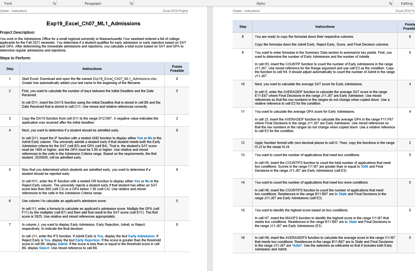
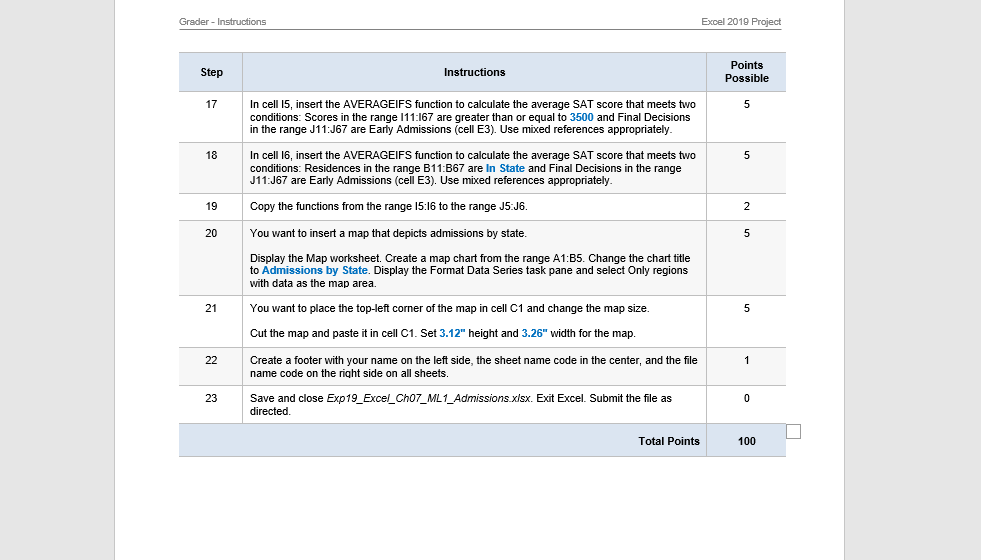
Font Paragraph Styles Editing Grader - Instructions :- Excel 2019 Project Grader - Instructions Excel 2019 Pro Step Instructions Points Possibl 8 You are ready to copy the formulas down their respective columns. 6 Exp19_Excel_Ch07_ML1_Admissions Project Description: You work in the Admissions Office for a small regional university in Massachusetts Your assistant entered a list of college applicants for the Fall 2021 semester. You determine if a student qualifies for early admission or early rejection based on SAT and GPA. After determining the immediate admissions and rejections, you calculate a total score based on SAT and GPA to determine regular admissions and rejections. Steps to Perform: Copy the formulas down the Admit Early, Reject Early, Score, and Final Decision columns 9 5 You want to enter formulas in the Summary Data section to summarize key points. First, you want to determine the number of Early Admissions and the number of Admits. In cell H3, insert the COUNTIF function to count the number of Early Admissions in the range J11:J67. Use mixed reference for the Range argument and use cell E3 as the condition. Copy the function to cell H4. It should adjust automatically to count the number of Admit in the range J11:J67 Step Instructions Points Possible 1 0 Start Excel. Download and open the file named Exp19_Excel_Ch07_ML1_Admissions.xlsx. Grader has automatically added your last name to the beginning of the filename. 10 Next, you want to calculate the average SAT score for Early Admissions 4 2 5 First, you want to calculate the number of days between the Initial Deadline and the Date Received. In cell D11, insert the DAYS function using the Initial Deadline that is stored in cell B8 and the Date Received that is stored in cell C11. Use mixed and relative references correctly. 11 In cell 13, enter the AVERAGEIF function to calculate the average SAT score in the range E11:E67 where Final Decisions in the range J11:J67 are Early Admission. Use mixed references so that the row numbers in the ranges do not change when copied down. Use a relative reference to cell E3 for the condition. You want to calculate the average GPA score for Early Admissions. In cell J3, insert the AVERAGEIF function to calculate the average GPA in the range F11:567 where Final Decisions in the range J11:J67 are Early Admission. Use mixed references so that the row numbers in the ranges do not change when copied down. Use a relative reference to cell E3 for the condition. 4 3 2 Copy the DAYS function from cell D11 to the range D12:067. A negative value indicates the application was received after the initial deadline. 4 4 Next, you want to determine if a student should be admitted early 8 12 In cell G11, insert the IF function with a nested AND function to display either Yes or No in the Admit Early column. The university admits a student early if that student meets both the Early Admission criteria for the SAT (cell B3) and GPA (cell B4). That is, the student's SAT score must be 1400 or higher, and the GPA must be 3.80 or higher. Use relative and mixed references to the cells in the Admission Criteria range. Based on the requirements, the first student, 2020005, will be admitted early Apply Number format with zero decimal places to cell 13. Then, copy the functions in the range 13:J3 to the range 14:J4. 2 13 You want to count the number of applications that meet two conditions. 5 In cell H5, insert the COUNTIFS function to count the total number of applications that meet two conditions: Scores in the range 111:167 are greater than or equal to 3500 and Final Decisions in the range J11:J67 are Early Admissions (cell E3). 5 5 8 14 You want to count the number of applications that meet two more conditions 5 In cell H6, insert the COUNTIFS function to count the number of applications that meet two conditions: Residences in the range B11:367 are In State and Final Decisions in the range J11:J67 are Early Admissions (cell E3) 6 5 Now that you determined which students are admitted early, you want to determine if a student should be rejected early. In cell H11, enter the IF function with a nested OR function to display either Yes or No in the Reject Early column. The university rejects a student early if that student has either an SAT score less than 800 (cell C3) or a GPA below 1.80 (cell C4). Use relative and mixed references to the cells in the Admission Criteria range. Use column 1 to calculate an applicant's admission score. In cell 111, enter a formula to calculate an applicant's admission score. Multiply the GPA (cell F11) by the multiplier (cell B7) and then add that result to the SAT score (cell E11). The first score is 3925. Use relative and mixed references appropriately. In column J, you want to display Early Admission, Early Rejection, Admit, or Reject, respectively, to indicate the final decision. In cell J11, enter the IFS function. If Admit Early is Yes, display the text Early Admission. If Reject Early is Yes, display the text Early Rejection. If the score is greater than the threshold score in cell B6, display Admit. If the score is less than or equal to the threshold score in cell B6, display Reject. Use mixed reference to cell B6. . 15 5 You want to identify the highest score based on two conditions. In cell H7, insert the MAXIFS function to identify the highest score in the range 111:167 that meets two conditions: Residences in the range B11:367 are In State and Final Decisions in the range J11:J67 are Early Admissions (E3). 7 8 16 5 In cell H8, insert the AVERAGEIFS function to calculate the average score in the range 111:167 that meets two conditions: Residences in the range B11:367 are in State and Final Decisions in the range J11:J67 are *Adm. Use the asterisks as wildcards so that it includes both Early Admission and Admit. Grader - Instructions Excel 2010 Project Step Instructions Points Possible 17 5 In cell 15, insert the AVERAGEIFS function to calculate the average SAT score that meets two conditions: Scores in the range 111:167 are greater than or equal to 3500 and Final Decisions in the range J11:J67 are Early Admissions (cell E3). Use mixed references appropriately 18 5 In cell 16, insert the AVERAGEIFS function to calculate the average SAT score that meets two conditions: Residences in the range B11:367 are in State and Final Decisions in the range J11:J67 are Early Admissions (cell E3). Use mixed references appropriately Copy the functions from the range 15:16 to the range J5:36. 19 2 20 5 You want to insert a map that depicts admissions by state. Display the Map worksheet. Create a map chart from the range A1:35. Change the chart title to Admissions by State. Display the Format Data Series task pane and select Only regions with data as the map area, 21 You want to place the top-left corner of the map in cell C1 and change the map size. 5 Cut the map and paste it in cell C1. Set 3.12" height and 3.26" width for the map. 22 1 Create a footer with your name on the left side, the sheet name code in the center, and the file name code on the right side on all sheets. 23 0 Save and close Exp19_Excel_Cho7_ML1_Admissions.xlsx. Exit Excel. Submit the file as directed Total Points 100 Font Paragraph Styles Editing Grader - Instructions :- Excel 2019 Project Grader - Instructions Excel 2019 Pro Step Instructions Points Possibl 8 You are ready to copy the formulas down their respective columns. 6 Exp19_Excel_Ch07_ML1_Admissions Project Description: You work in the Admissions Office for a small regional university in Massachusetts Your assistant entered a list of college applicants for the Fall 2021 semester. You determine if a student qualifies for early admission or early rejection based on SAT and GPA. After determining the immediate admissions and rejections, you calculate a total score based on SAT and GPA to determine regular admissions and rejections. Steps to Perform: Copy the formulas down the Admit Early, Reject Early, Score, and Final Decision columns 9 5 You want to enter formulas in the Summary Data section to summarize key points. First, you want to determine the number of Early Admissions and the number of Admits. In cell H3, insert the COUNTIF function to count the number of Early Admissions in the range J11:J67. Use mixed reference for the Range argument and use cell E3 as the condition. Copy the function to cell H4. It should adjust automatically to count the number of Admit in the range J11:J67 Step Instructions Points Possible 1 0 Start Excel. Download and open the file named Exp19_Excel_Ch07_ML1_Admissions.xlsx. Grader has automatically added your last name to the beginning of the filename. 10 Next, you want to calculate the average SAT score for Early Admissions 4 2 5 First, you want to calculate the number of days between the Initial Deadline and the Date Received. In cell D11, insert the DAYS function using the Initial Deadline that is stored in cell B8 and the Date Received that is stored in cell C11. Use mixed and relative references correctly. 11 In cell 13, enter the AVERAGEIF function to calculate the average SAT score in the range E11:E67 where Final Decisions in the range J11:J67 are Early Admission. Use mixed references so that the row numbers in the ranges do not change when copied down. Use a relative reference to cell E3 for the condition. You want to calculate the average GPA score for Early Admissions. In cell J3, insert the AVERAGEIF function to calculate the average GPA in the range F11:567 where Final Decisions in the range J11:J67 are Early Admission. Use mixed references so that the row numbers in the ranges do not change when copied down. Use a relative reference to cell E3 for the condition. 4 3 2 Copy the DAYS function from cell D11 to the range D12:067. A negative value indicates the application was received after the initial deadline. 4 4 Next, you want to determine if a student should be admitted early 8 12 In cell G11, insert the IF function with a nested AND function to display either Yes or No in the Admit Early column. The university admits a student early if that student meets both the Early Admission criteria for the SAT (cell B3) and GPA (cell B4). That is, the student's SAT score must be 1400 or higher, and the GPA must be 3.80 or higher. Use relative and mixed references to the cells in the Admission Criteria range. Based on the requirements, the first student, 2020005, will be admitted early Apply Number format with zero decimal places to cell 13. Then, copy the functions in the range 13:J3 to the range 14:J4. 2 13 You want to count the number of applications that meet two conditions. 5 In cell H5, insert the COUNTIFS function to count the total number of applications that meet two conditions: Scores in the range 111:167 are greater than or equal to 3500 and Final Decisions in the range J11:J67 are Early Admissions (cell E3). 5 5 8 14 You want to count the number of applications that meet two more conditions 5 In cell H6, insert the COUNTIFS function to count the number of applications that meet two conditions: Residences in the range B11:367 are In State and Final Decisions in the range J11:J67 are Early Admissions (cell E3) 6 5 Now that you determined which students are admitted early, you want to determine if a student should be rejected early. In cell H11, enter the IF function with a nested OR function to display either Yes or No in the Reject Early column. The university rejects a student early if that student has either an SAT score less than 800 (cell C3) or a GPA below 1.80 (cell C4). Use relative and mixed references to the cells in the Admission Criteria range. Use column 1 to calculate an applicant's admission score. In cell 111, enter a formula to calculate an applicant's admission score. Multiply the GPA (cell F11) by the multiplier (cell B7) and then add that result to the SAT score (cell E11). The first score is 3925. Use relative and mixed references appropriately. In column J, you want to display Early Admission, Early Rejection, Admit, or Reject, respectively, to indicate the final decision. In cell J11, enter the IFS function. If Admit Early is Yes, display the text Early Admission. If Reject Early is Yes, display the text Early Rejection. If the score is greater than the threshold score in cell B6, display Admit. If the score is less than or equal to the threshold score in cell B6, display Reject. Use mixed reference to cell B6. . 15 5 You want to identify the highest score based on two conditions. In cell H7, insert the MAXIFS function to identify the highest score in the range 111:167 that meets two conditions: Residences in the range B11:367 are In State and Final Decisions in the range J11:J67 are Early Admissions (E3). 7 8 16 5 In cell H8, insert the AVERAGEIFS function to calculate the average score in the range 111:167 that meets two conditions: Residences in the range B11:367 are in State and Final Decisions in the range J11:J67 are *Adm. Use the asterisks as wildcards so that it includes both Early Admission and Admit. Grader - Instructions Excel 2010 Project Step Instructions Points Possible 17 5 In cell 15, insert the AVERAGEIFS function to calculate the average SAT score that meets two conditions: Scores in the range 111:167 are greater than or equal to 3500 and Final Decisions in the range J11:J67 are Early Admissions (cell E3). Use mixed references appropriately 18 5 In cell 16, insert the AVERAGEIFS function to calculate the average SAT score that meets two conditions: Residences in the range B11:367 are in State and Final Decisions in the range J11:J67 are Early Admissions (cell E3). Use mixed references appropriately Copy the functions from the range 15:16 to the range J5:36. 19 2 20 5 You want to insert a map that depicts admissions by state. Display the Map worksheet. Create a map chart from the range A1:35. Change the chart title to Admissions by State. Display the Format Data Series task pane and select Only regions with data as the map area, 21 You want to place the top-left corner of the map in cell C1 and change the map size. 5 Cut the map and paste it in cell C1. Set 3.12" height and 3.26" width for the map. 22 1 Create a footer with your name on the left side, the sheet name code in the center, and the file name code on the right side on all sheets. 23 0 Save and close Exp19_Excel_Cho7_ML1_Admissions.xlsx. Exit Excel. Submit the file as directed Total Points 100

 Type or paste question here


