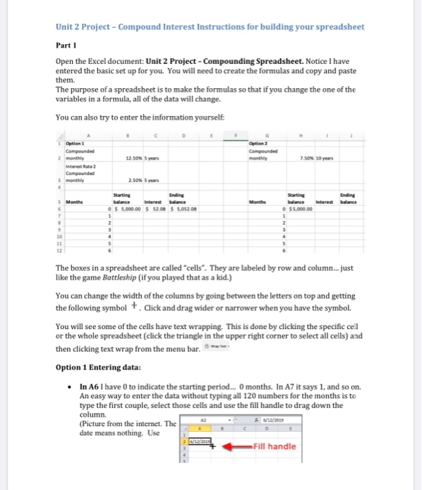
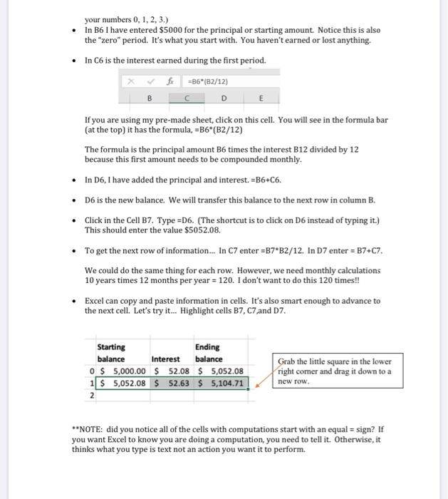
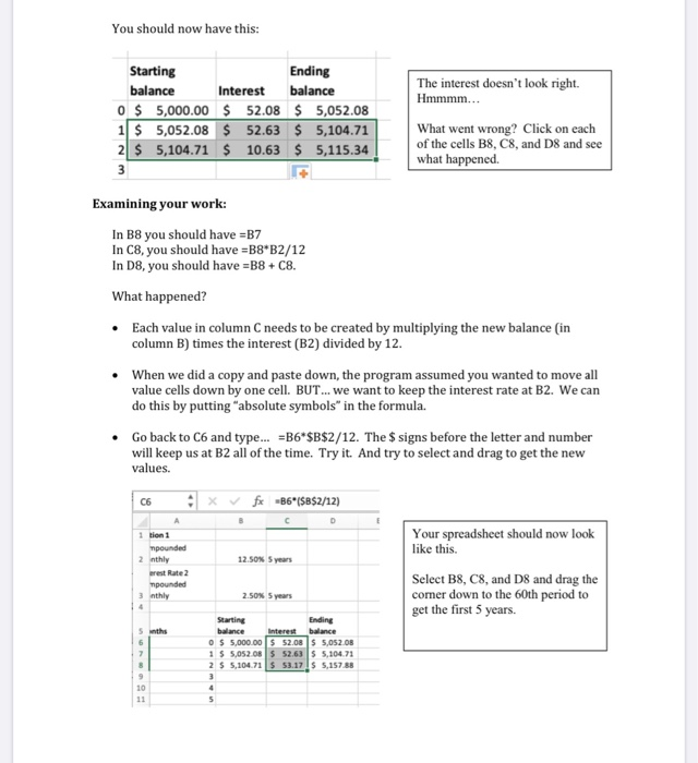
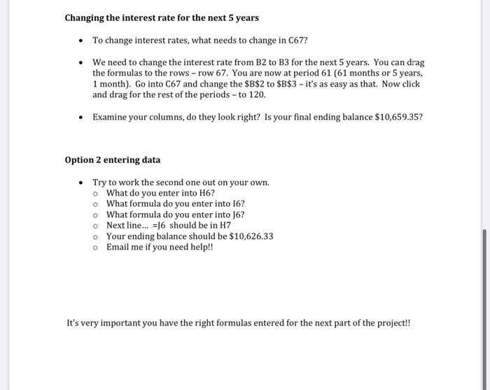
Unit 2 Project - Compound Interest Instructions for building your spreadsheet Part 1 Open the Excel document: Unit 2 Project - Compounding Spreadsheet. Notice I have entered the basic set up for you. You will need to create the formulas and copy and paste them. The purpose of a spreadsheet is to make the formulas so that if you change the one of the variables in a formula, all of the data will change. You can also try to enter the information yourself Option 1 Compounded 2 monthly Interest Rate 2 Compounded Option 2 Compounded monthly 12.50N 5 years 7.50N 10 years 2.50% 5 years Ending Interest balance Month 5 Months 6 7 Starting $5.000.00 Interest balance O $5,000.00 $ 52.08 $ 5.02.08 2 3 2 10 11 12 The boxes in a spreadsheet are called "cells". They are labeled by row and column...just like the game Battleship (if you played that as a kid.) You can change the width of the columns by going between the letters on top and getting the following symbol + Click and drag wider or narrower when you have the symbol. You will see some of the cells have text wrapping. This is done by clicking the specific cell or the whole spreadsheet (click the triangle in the upper right corner to select all cells) and then clicking text wrap from the menu bar. Option 1 Entering data: In A6 I have 0 to indicate the starting period... O months. In A7 it says 1, and so on. An easy way to enter the data without typing all 120 numbers for the months is to type the first couple, select those cells and use the fill handle to drag down the column (Picture from the internet. The 6/12/2019 date means nothing. Use Fill handle your numbers 0, 1, 2, 3.) In B6 I have entered $5000 for the principal or starting amount. Notice this is also the "zero" period. It's what you start with. You haven't earned or lost anything. In C6 is the interest earned during the first period. fo=B6* (B2/12) E If you are using my pre-made sheet, click on this cell. You will see in the formula bar (at the top) it has the formula, =B6*(B2/12) The formula is the principal amount B6 times the interest B12 divided by 12 because this first amount needs to be compounded monthly. In D6, I have added the principal and interest. =B6+C6. D6 is the new balance. We will transfer this balance to the next row in column B. Click in the Cell B7. Type =D6. (The shortcut is to click on D6 instead of typing it.) This should enter the value $5052.08. To get the next row of information... In C7 enter =B7*B2/12. In D7 enter = B7+07. We could do the same thing for each row. However, we need monthly calculations 10 years times 12 months per year = 120. I don't want to do this 120 times!! Excel can copy and paste information in cells. It's also smart enough to advance to the next cell. Let's try it... Highlight cells B7, C7,and D7. balance Starting Ending balance Interest O $5,000.00 $ 52.08 $ 5,052.08 1$ 5,052.08 $ 52.63 $ 5,104.71 2 Grab the little square in the lower right comer and drag it down to a new row. **NOTE: did you notice all of the cells with computations start with an equal = sign? If you want Excel to know you are doing a computation, you need to tell it. Otherwise, it thinks what you type is text not an action you want it to perform. You should now have this: Starting Ending balance Interest balance 0 $ 5,000.00 $ 52.08 $ 5,052.08 1 $ 5,052.08 $ 52.63 $ 5,104.71 2 $ 5,104.71 $ 10.63 $ 5,115.34 3 The interest doesn't look right. Hmmmm... What went wrong? Click on each of the cells B8, C8, and D8 and see what happened. Examining your work: In B8 you should have =B7 In C8, you should have =B8*B2/12 In D8, you should have =B8 + C8. What happened? Each value in column C needs to be created by multiplying the new balance in column B) times the interest (B2) divided by 12. When we did a copy and paste down, the program assumed you wanted to move all value cells down by one cell. BUT... We want to keep the interest rate at B2. We can do this by putting "absolute symbols in the formula. Go back to C6 and type... =B6*$B$2/12. The $ signs before the letter and number will keep us at B2 all of the time. Try it. And try to select and drag to get the new values. C6 * fx B6*($B$2/12) B D A 1 tion 1 mpounded 2 nthly rest Rate 2 mpounded 3 nthly 12.50N 5 years Your spreadsheet should now look like this. Select B8, C8, and D8 and drag the comer down to the 60th period to get the first 5 years. 2.SON 5 years 5 with 7 Starting Ending balance Interest balance O $5,000.00 $ 52.08 $ 5,052.08 1 $ 5,052.08 S 52.63 5.104.71 2 $ 5,104.71 53.175 5,157,88 3 4 5 9 10 11 Changing the interest rate for the next 5 years To change interest rates, what needs to change in C67? We need to change the interest rate from B2 to B3 for the next 5 years. You can drag the formulas to the rows - row 67. You are now at period 61 (61 months or 5 years, 1 month). Go into C67 and change the $B$2 to $B$3 - it's as easy as that. Now click and drag for the rest of the periods - to 120. Examine your columns, do they look right? Is your final ending balance $10,659.35? Option 2 entering data Try to work the second one out on your own. o What do you enter into H6? o What formula do you enter into 16? o What formula do you enter into J6? o Next line... =J6 should be in H7 Your ending balance should be $10,626.33 Email me if you need help!! It's very important you have the right formulas entered for the next part of the project!! Unit 2 Project - Compound Interest Instructions for building your spreadsheet Part 1 Open the Excel document: Unit 2 Project - Compounding Spreadsheet. Notice I have entered the basic set up for you. You will need to create the formulas and copy and paste them. The purpose of a spreadsheet is to make the formulas so that if you change the one of the variables in a formula, all of the data will change. You can also try to enter the information yourself Option 1 Compounded 2 monthly Interest Rate 2 Compounded Option 2 Compounded monthly 12.50N 5 years 7.50N 10 years 2.50% 5 years Ending Interest balance Month 5 Months 6 7 Starting $5.000.00 Interest balance O $5,000.00 $ 52.08 $ 5.02.08 2 3 2 10 11 12 The boxes in a spreadsheet are called "cells". They are labeled by row and column...just like the game Battleship (if you played that as a kid.) You can change the width of the columns by going between the letters on top and getting the following symbol + Click and drag wider or narrower when you have the symbol. You will see some of the cells have text wrapping. This is done by clicking the specific cell or the whole spreadsheet (click the triangle in the upper right corner to select all cells) and then clicking text wrap from the menu bar. Option 1 Entering data: In A6 I have 0 to indicate the starting period... O months. In A7 it says 1, and so on. An easy way to enter the data without typing all 120 numbers for the months is to type the first couple, select those cells and use the fill handle to drag down the column (Picture from the internet. The 6/12/2019 date means nothing. Use Fill handle your numbers 0, 1, 2, 3.) In B6 I have entered $5000 for the principal or starting amount. Notice this is also the "zero" period. It's what you start with. You haven't earned or lost anything. In C6 is the interest earned during the first period. fo=B6* (B2/12) E If you are using my pre-made sheet, click on this cell. You will see in the formula bar (at the top) it has the formula, =B6*(B2/12) The formula is the principal amount B6 times the interest B12 divided by 12 because this first amount needs to be compounded monthly. In D6, I have added the principal and interest. =B6+C6. D6 is the new balance. We will transfer this balance to the next row in column B. Click in the Cell B7. Type =D6. (The shortcut is to click on D6 instead of typing it.) This should enter the value $5052.08. To get the next row of information... In C7 enter =B7*B2/12. In D7 enter = B7+07. We could do the same thing for each row. However, we need monthly calculations 10 years times 12 months per year = 120. I don't want to do this 120 times!! Excel can copy and paste information in cells. It's also smart enough to advance to the next cell. Let's try it... Highlight cells B7, C7,and D7. balance Starting Ending balance Interest O $5,000.00 $ 52.08 $ 5,052.08 1$ 5,052.08 $ 52.63 $ 5,104.71 2 Grab the little square in the lower right comer and drag it down to a new row. **NOTE: did you notice all of the cells with computations start with an equal = sign? If you want Excel to know you are doing a computation, you need to tell it. Otherwise, it thinks what you type is text not an action you want it to perform. You should now have this: Starting Ending balance Interest balance 0 $ 5,000.00 $ 52.08 $ 5,052.08 1 $ 5,052.08 $ 52.63 $ 5,104.71 2 $ 5,104.71 $ 10.63 $ 5,115.34 3 The interest doesn't look right. Hmmmm... What went wrong? Click on each of the cells B8, C8, and D8 and see what happened. Examining your work: In B8 you should have =B7 In C8, you should have =B8*B2/12 In D8, you should have =B8 + C8. What happened? Each value in column C needs to be created by multiplying the new balance in column B) times the interest (B2) divided by 12. When we did a copy and paste down, the program assumed you wanted to move all value cells down by one cell. BUT... We want to keep the interest rate at B2. We can do this by putting "absolute symbols in the formula. Go back to C6 and type... =B6*$B$2/12. The $ signs before the letter and number will keep us at B2 all of the time. Try it. And try to select and drag to get the new values. C6 * fx B6*($B$2/12) B D A 1 tion 1 mpounded 2 nthly rest Rate 2 mpounded 3 nthly 12.50N 5 years Your spreadsheet should now look like this. Select B8, C8, and D8 and drag the comer down to the 60th period to get the first 5 years. 2.SON 5 years 5 with 7 Starting Ending balance Interest balance O $5,000.00 $ 52.08 $ 5,052.08 1 $ 5,052.08 S 52.63 5.104.71 2 $ 5,104.71 53.175 5,157,88 3 4 5 9 10 11 Changing the interest rate for the next 5 years To change interest rates, what needs to change in C67? We need to change the interest rate from B2 to B3 for the next 5 years. You can drag the formulas to the rows - row 67. You are now at period 61 (61 months or 5 years, 1 month). Go into C67 and change the $B$2 to $B$3 - it's as easy as that. Now click and drag for the rest of the periods - to 120. Examine your columns, do they look right? Is your final ending balance $10,659.35? Option 2 entering data Try to work the second one out on your own. o What do you enter into H6? o What formula do you enter into 16? o What formula do you enter into J6? o Next line... =J6 should be in H7 Your ending balance should be $10,626.33 Email me if you need help!! It's very important you have the right formulas entered for the next part of the project