use excel format please

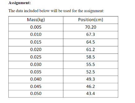
Click on the upper left corner of the spreadsheet to select the entire spreadsheet and set font to Times New Roman and size 14. 2. Your excel spreadsheet must start with a title centered across all the columns (use the merge and center button for this). Use Excel Exercise as the title. 3. Use the first two columns in Sheet1 to enter the data above. Use column A for the mass and column B for the Position. Each column must have the title included with the data. All data and titles must be centered. All titles must be Bold. 4. Title column C Position (m) 5. In column C convert all the values in column B from centimeters to meters. Use this by using a formula that divides each cell in column B by 100. Do not use your calculator. You must use a formula in excel to receive credit for this step.

6. Title Column D Stretch (m) 7. Fill the cells in column D with a formula that subtracts the values of column C from the first value of the position in column C. Make sure that you anchor the first cell row by using a dollar sign. Example: C$3-C3. The value in cell D3 will be zero. 8. Select cell D3 by clicking on it and release. Move the cursor to the lower right corner of the cell D3 (do not click while doing this). Notice that the cursor turns into a skinny black cross. Depress the button and drag down to cell D12. The formula should be copied down using the values in column C as the input. 9. In cell H2 type gravity (m/s^2) (just the words in bold, do not include the quotes). 10. In cell H3 type 9.80 11. Tile Column E Force (N) 12. Fill column E with the multiplication of the values in column A (mass) times the value in cell H3. This is the weight. Make sure that you use the dollar sign ($) to anchor the value of g in cell H3. See step 7 for help. 13. Format all the data to three decimal places and set all the columns width to display the data correctly. 14. Graph Column D (x-axis) vs. Column E (y axis) by selecting Columns D and E. Click the Insert Tab in the excel ribbon and in the Charts Group, click the Scatter button. 15. Make sure that the graph is in its own page and it is not embedded in the spreadsheet. 16. Include a linear trendline for the data. Also, include the equation of the trendline. 17. Consult the proper graphing handout in the website to complete your graph (link). 18. Use Simple Harmonic Motion as the title of the chart. 19. Use Stretch (m) for the x-axis tile and Force (N) for the y-axis title. 20. Compare your work with the sample PDF included in the lab module.

The data included below will be used for the assignment