USE Mathematica


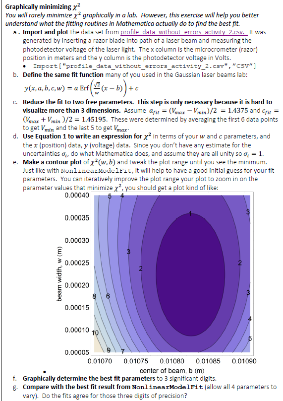
Graphically minimizing x You will rarely minimize x2 graphically in a lab. However, this exercise will help you better understand what the fitting routines in Mathematica actually do to find the best fit. a. Import and plot the data set from profile data without errors activity 2.csv. It was generated by inserting a razor blade into path of a laser beam and measuring the photodetector voltage of the laser light. The x column is the microcrometer (razor) position in meters and the y column is the photodetector voltage in Volts. Import["profile_data_without_errors_activity_2.csv","CSV"] b. Define the same fit function many of you used in the Gaussian laser beams lab: y(x, a, b,c,w) = a Erf((x - b)) + C. Reduce the fit to two free parameters. This step is only necessary because it is hard to visualize more than 3 dimensions. Assume a fit = (Vmax - Vmin)/2 = 1.4375 and Cfit = (Vmax + V min)/2 = 1.45195. These were determined by averaging the first 6 data points to get Vmin and the last 5 to get Vmax. d. Use Equation 1 to write an expression for x? in terms of your w and c parameters, and the x (position) data, y (voltage) data. Since you don't have any estimate for the uncertainties o, do what Mathematica does, and assume they are all unity so a; = 1. e. Make a contour plot of x-(w,b) and tweak the plot range until you see the minimum. Just like with NonlinearModelFit, it will help to have a good initial guess for your fit parameters. You can iteratively improve the plot range your plot to zoom in on the parameter values that minimize x?, you should get a plot kind of like: 0.00040 0.00035 0.00030 0.00025 beam width, w (m) 0.00020 8 0.00015 0.00010 10 0.00005 7 0.01070 0.01075 0.01080 0.01085 0.01090 center of beam, b (m) f. Graphically determine the best fit parameters to 3 significant digits. g. Compare with the best fit result from NonlinearModelFit (allow all 4 parameters to vary). Do the fits agree for those three digits of precision? A 0.01016 0.010211 0.010262 0.010312 0.010363 0.010414 0.010465 0.010516 0.010566 0.010617 0.010668 0.010719 0.01077 0.01082 0.010871 0.010922 0.010973 0.011024 0.011074 0.011125 0.011176 0.011227 0.011278 0.011328 0.011379 0.01143 B 0.014 0.014 0.014 0.015 0.015 0.015 0.016 0.017 0.026 0.06 0.176 0.46 0.849 1.364 1.971 2.41 2.703 2.795 2.861 2.879 2.884 2.894 2.889 2.886 2.89 2.888 Graphically minimizing x You will rarely minimize x2 graphically in a lab. However, this exercise will help you better understand what the fitting routines in Mathematica actually do to find the best fit. a. Import and plot the data set from profile data without errors activity 2.csv. It was generated by inserting a razor blade into path of a laser beam and measuring the photodetector voltage of the laser light. The x column is the microcrometer (razor) position in meters and the y column is the photodetector voltage in Volts. Import["profile_data_without_errors_activity_2.csv","CSV"] b. Define the same fit function many of you used in the Gaussian laser beams lab: y(x, a, b,c,w) = a Erf((x - b)) + C. Reduce the fit to two free parameters. This step is only necessary because it is hard to visualize more than 3 dimensions. Assume a fit = (Vmax - Vmin)/2 = 1.4375 and Cfit = (Vmax + V min)/2 = 1.45195. These were determined by averaging the first 6 data points to get Vmin and the last 5 to get Vmax. d. Use Equation 1 to write an expression for x? in terms of your w and c parameters, and the x (position) data, y (voltage) data. Since you don't have any estimate for the uncertainties o, do what Mathematica does, and assume they are all unity so a; = 1. e. Make a contour plot of x-(w,b) and tweak the plot range until you see the minimum. Just like with NonlinearModelFit, it will help to have a good initial guess for your fit parameters. You can iteratively improve the plot range your plot to zoom in on the parameter values that minimize x?, you should get a plot kind of like: 0.00040 0.00035 0.00030 0.00025 beam width, w (m) 0.00020 8 0.00015 0.00010 10 0.00005 7 0.01070 0.01075 0.01080 0.01085 0.01090 center of beam, b (m) f. Graphically determine the best fit parameters to 3 significant digits. g. Compare with the best fit result from NonlinearModelFit (allow all 4 parameters to vary). Do the fits agree for those three digits of precision? A 0.01016 0.010211 0.010262 0.010312 0.010363 0.010414 0.010465 0.010516 0.010566 0.010617 0.010668 0.010719 0.01077 0.01082 0.010871 0.010922 0.010973 0.011024 0.011074 0.011125 0.011176 0.011227 0.011278 0.011328 0.011379 0.01143 B 0.014 0.014 0.014 0.015 0.015 0.015 0.016 0.017 0.026 0.06 0.176 0.46 0.849 1.364 1.971 2.41 2.703 2.795 2.861 2.879 2.884 2.894 2.889 2.886 2.89 2.888


