USE MATLAB:

plotdata

computecost

gradientdescent

main (don't change)

%% Machine Learning Online Class - Linear Regression

% Instructions

% ------------

%

% This file contains code that helps you get started on the

% linear exercise. You will need to complete the following functions

% in this exericse:

%

% plotData.m

% gradientDescent.m

% computeCost.m

%

% For this exercise, you will not need to change any code in this file,

% or any other files other than those mentioned above.

%

% x refers to the population size in 10,000s

% y refers to the profit in $10,000s

%

%% Initialization

clear ; close all; clc

%% ======================= Part 1: Plotting =======================

fprintf('Plotting Data ... ')

data = load('data1.txt');

X = data(:, 1); y = data(:, 2);

m = length(y); % number of training examples

% Plot Data

% Note: You have to complete the code in plotData.m

plotData(X, y);

fprintf('Program paused. Press enter to continue. ');

pause;

%% =================== Part 2: Cost function ===================

X = [ones(m, 1), data(:,1)]; % Add a column of ones to x

theta = zeros(2, 1); % initialize fitting parameters

fprintf(' Testing the cost function ... ')

% compute and display initial cost

J = computeCost(X, y, theta);

fprintf('With theta = [0 ; 0] Cost computed = %f ', J);

fprintf('Expected cost value (approx) 32.07 ');

% further testing of the cost function

J = computeCost(X, y, [-1 ; 2]);

fprintf(' With theta = [-1 ; 2] Cost computed = %f ', J);

fprintf('Expected cost value (approx) 54.24 ');

fprintf('Program paused. Press enter to continue. ');

pause;

%% =================== Part 3: Gradient descent ===================

% Some gradient descent settings

iterations = 1500;

alpha = 0.01;

fprintf(' Running Gradient Descent ... ')

% run gradient descent

theta = gradientDescent(X, y, theta, alpha, iterations);

% print theta to screen

fprintf('Theta found by gradient descent: ');

fprintf('%f ', theta);

fprintf('Expected theta values (approx) ');

fprintf(' -3.6303 1.1664 ');

% Plot the linear fit

hold on; % keep previous plot visible

plot(X(:,2), X*theta, '-')

legend('Training data', 'Linear regression')

hold off % don't overlay any more plots on this figure

% Predict values for population sizes of 35,000 and 70,000

predict1 = [1, 3.5] *theta;

fprintf('For population = 35,000, we predict a profit of %f ',...

predict1*10000);

predict2 = [1, 7] * theta;

fprintf('For population = 70,000, we predict a profit of %f ',...

predict2*10000);

fprintf('Program paused. Press enter to continue. ');

pause;

%% ============= Part 4: Visualizing J(theta_0, theta_1) =============

fprintf('Visualizing J(theta_0, theta_1) ... ')

% Grid over which we will calculate J

theta0_vals = linspace(-10, 10, 100);

theta1_vals = linspace(-1, 4, 100);

% initialize J_vals to a matrix of 0's

J_vals = zeros(length(theta0_vals), length(theta1_vals));

% Fill out J_vals

for i = 1:length(theta0_vals)

for j = 1:length(theta1_vals)

t = [theta0_vals(i); theta1_vals(j)];

J_vals(i,j) = computeCost(X, y, t);

end

end

% Because of the way meshgrids work in the surf command, we need to

% transpose J_vals before calling surf, or else the axes will be flipped

J_vals = J_vals';

% Surface plot

figure;

surf(theta0_vals, theta1_vals, J_vals)

xlabel('\theta_0'); ylabel('\theta_1');

% Contour plot

figure;

% Plot J_vals as 15 contours spaced logarithmically between 0.01 and 100

contour(theta0_vals, theta1_vals, J_vals, logspace(-2, 3, 20))

xlabel('\theta_0'); ylabel('\theta_1');

hold on;

plot(theta(1), theta(2), 'rx', 'MarkerSize', 10, 'LineWidth', 2);

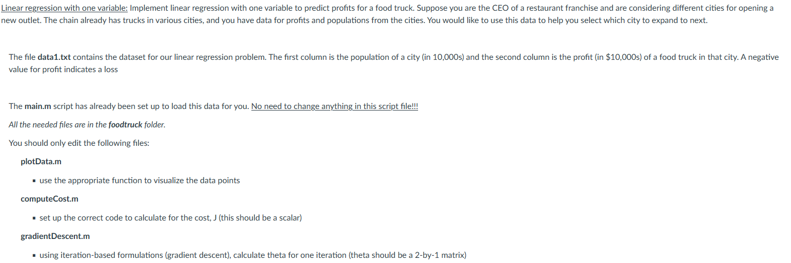
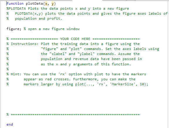
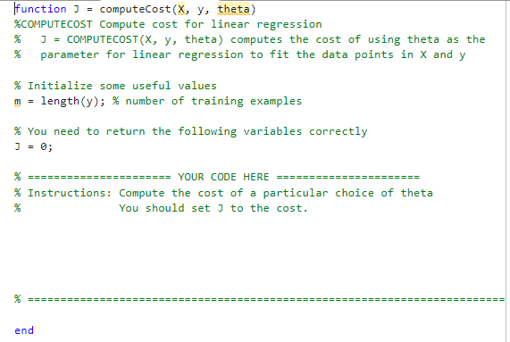
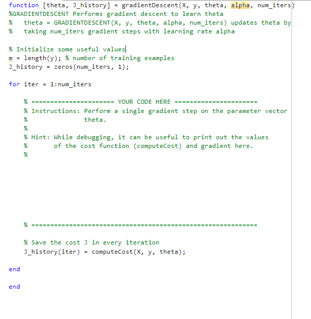
value for profit indicates a loss The main.m script has already been set up to load this data for you. No need to change anything in this script file!!! All the needed files are in the foodtruck folder. You should only edit the following files: plotData.m - use the appropriate function to visualize the data points computeCost.m - set up the correct code to calculate for the cost, J (this should be a scalar) gradientDescent.m - using iteration-based formulations (gradient descent), calculate theta for one iteration (theta should be a 2-by-1 matrix) \% PLOTDATA (x,y) plots the data points and gives the figure axes labels \% population and profit. figure; \% open a new figure window \% Instructions: Plot the training data into a figure using the \% "figure" and "plot" commands. Set the axes labels using the "xlabel" and "ylabel" commands. Assume the population and revenue data have been passed in as the x and y arguments of this function. \% Hint: You can use the 'rx' option with plot to have the markers \% appear as red crosses. Furthermore, you can make the \% markers larger by using plot (..., 'rx', 'MarkerSize', 10); ffunction J = computeCost ( X,y, theta) \%COMPUTECOST Compute cost for linear regression %J=COMPUTECOST(x,y, theta) computes the cost of using theta as the % parameter for linear regression to fit the data points in X and y \% Initialize some useful values m= length (y);% number of training examples \% You need to return the following variables correctly J=0; \% ====================== YOUR CODE HERE ====================== \% Instructions: Compute the cost of a particular choice of theta \% You should set J to the cost. \% ==0==0=0=0=0=0=0=0=0=0=0=0=0=0=0=0=0=0=0=0=0=0=0=0=0==0=0=0=0=0=0=0=0=0 end function [theta, J_history] = gradientDescent(X, y, theta, alpha, num_iters \%GRADIENTDESCENT Performs gradient descent to learn theta % theta = GRADIENTDESCENT(X, y, theta, alpha, num_iters) updates theta by \% taking num_iters gradient steps with learning rate alpha \% Initialize some useful values| m= length(y); \% number of training examples J_history = zeros(num_iters, 1); for iter = 1:num_iters \% ===================== YOUR CoDE HERE ====================== \% Instructions: Perform a single gradient step on the parameter vector \% \% theta. \% Hint: While debugging, it can be useful to print out the values \% \% of the cost function (computeCost) and gradient here. \% Save the cost J in every iteration J_history (iter) = computeCost (X,y, theta); end end