use question 4 and data for question 4

to answer question 6

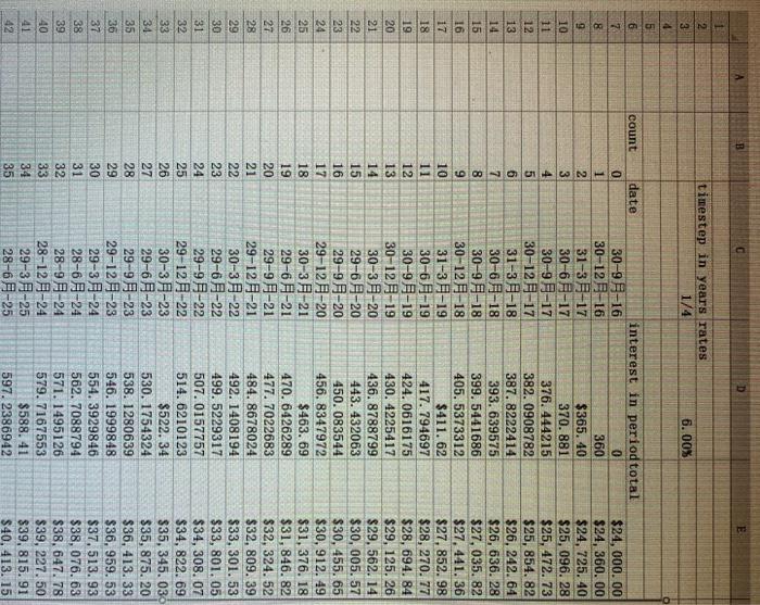
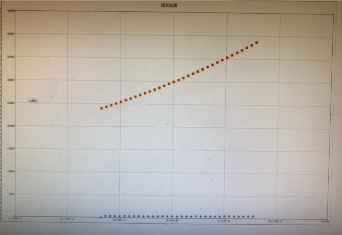
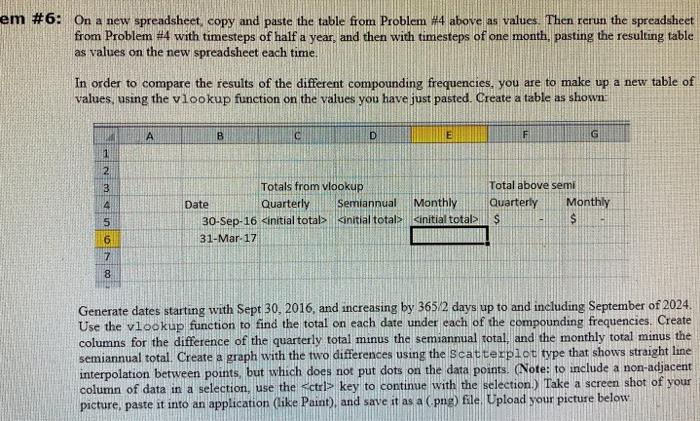
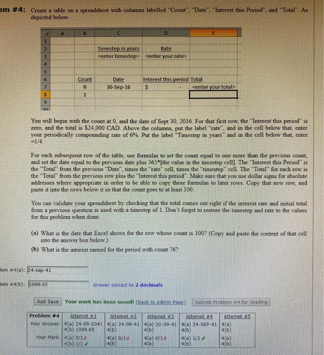
em #4: Create a table on a spreadsheet with columns labelled "Count", "Date". "Interest this period", and "Total". As depicted below A B D E 1 2 3 Timestep in years Rate center timestepsenter your rate> 4 5 Count 0 6 7 8 9 Date 30-Sep-16 Interest this period Total $ center your total 1 10 You will begin with the count at 0, and the date of Sept 30, 2016. For that first row, the "Interest this period" is zero, and the total is $24,000 CAD. Above the columns, put the label "rate", and in the cell below that, enter your periodically compounding rate of 6% Put the label "Timestep in years and in the cell below that, enter =1/4 For each subsequent row of the table, use formulas to set the count equal to one more than the previous count, and set the date equal to the previous date plus 365*[the value in the timestep cell]. The "Interest this period" is the "Total" from the previous "Date", times the "rate" cell times the "timestep" cell. The "Total" for each row is the "Total" from the previous row plus the "Interest this period". Make sure that you use dollar signs for absolute addresses where appropriate in order to be able to copy these formulas to later rows. Copy that new row, and paste it into the rows below it so that the count goes to at least 100 You can validate your spreadsheet by checking that the total comes out right if the interest rate and initial total from a previous question is used with a timestep of 1. Don't forget to restore the timestep and rate to the values for this problem when done (a) What is the date that Excel shows for the row whose count is 100? (Copy and paste the content of that cell into the answer box below.) (b) What is the interest eated for the period with count 76? Hem #4(a): 24-sep-41 Hem #4(b): 1099.65 Answer correct to 2 decimals Just Save Your work has been saved! (Back to Admin Page Submit Problem #4 for Grading Problem #4 Attemote Attempt 2 Attempt Attempt 24 Attempt Your Answer: 42) 24-09-2041 4(a) 24.09.41 4(a) 30-09-41 4() 24-SEP-41 4(a) 4(b) 1099.65 4(b) 406) 4(b) 4(1) Your Mark: 4(a) 0/1x 4(a) 0/EX 4(a) 0/1X 4(a) 1/1 4(a) 4(b) 1/1 4(b) 466 4(b) 416) A E (1) D 2 3 timestep in years rates 14 6.00% | count date 0 1 E 1 4 5 10 11 12 13 14 15 16 17 18 19 20 21 12 23 24 25 26 27 28 29 3 1 32 38 34 35 36 37 38 39 40 AL 2 9 11 11 12 13 14 15 16 17 18 19 20 21 22 23 24 25 26 27 28 29 36 31 interest in period total 30-9-16 16: 30-12-16 360 31-3-17 365.40 30-6-17 370.881 30-9-17 376.444215 30-12-17 382.9908782 313-18 387,8222414 30-6-18 393,639575 30-9-18 399,5441686 30-12-18 405.5373312 31-3-19 411.62 30-619 417.794697 30-9-19 424,9616175 30-12-19 430.4225417 303-20 436.8788799 29-6-20 43.432063 29-9-20 450.083544 29-12-20 456,8347972 30 3-21 $453.69 29-6-21 470.6426289 29-9-21 477,7022683 29-12-21 44,8678024 30-3-22 492.1408194 29-6-22 499.522931 29-9-22 507.0157757 29-12-22 514.6210123 30-3-23 $522.34 29-6-23 530.1754324 29-9-23 538.1280639 29-12-23 546.1999848 29-3-24 554,3929846 28-6-24 562,7088794 28-9-24 571.1495126 28-12-24 579.7167553 29-3-25 $588.41 28-6-25 597.2386942 $24.000.00 24.360.00 $24.725.40 $25,096.28 25,472.73 $25, 854.82 $26, 242.64 $26,536.28 $27,035.82 27.441.36 $27, 852.98 28, 270.7 28,694.84 29.125.26 $29,562.14 $30,005.57 $30,455.65 30,912.49 $31,376.18 $31, 846.82 $32,324.52 $32,809.39 $33,301.53 $33,801.05 $34,308.07 34,822.69 35,345.03. $35,875.20 $35:413.33 $36.959.53 $37,513.93 $38, 076.13 $38,647.78 $39 227,50 539.815.91 40 4135 32 33 34 35 E-ci -- 2001 BE 000 em #6: On a new spreadsheet, copy and paste the table from Problem #4 above as values. Then rerun the spreadsheet from Problem #4 with timesteps of half a year, and then with timesteps of one month, pasting the resulting table as values on the new spreadsheet each time In order to compare the results of the different compounding frequencies, you are to make up a new table of values, using the vlookup function on the values you have just pasted. Create a table as shown: B C D E F G 1 2 3 4 Totals from vlookup Date Quarterly Semiannual Monthly 30-Sep-16 key to continue with the selection.) Take a screen shot of your picture, paste it into an application (like Paint), and save it as a png) file. Upload your picture below em #4: Create a table on a spreadsheet with columns labelled "Count", "Date". "Interest this period", and "Total". As depicted below A B D E 1 2 3 Timestep in years Rate center timestepsenter your rate> 4 5 Count 0 6 7 8 9 Date 30-Sep-16 Interest this period Total $ center your total 1 10 You will begin with the count at 0, and the date of Sept 30, 2016. For that first row, the "Interest this period" is zero, and the total is $24,000 CAD. Above the columns, put the label "rate", and in the cell below that, enter your periodically compounding rate of 6% Put the label "Timestep in years and in the cell below that, enter =1/4 For each subsequent row of the table, use formulas to set the count equal to one more than the previous count, and set the date equal to the previous date plus 365*[the value in the timestep cell]. The "Interest this period" is the "Total" from the previous "Date", times the "rate" cell times the "timestep" cell. The "Total" for each row is the "Total" from the previous row plus the "Interest this period". Make sure that you use dollar signs for absolute addresses where appropriate in order to be able to copy these formulas to later rows. Copy that new row, and paste it into the rows below it so that the count goes to at least 100 You can validate your spreadsheet by checking that the total comes out right if the interest rate and initial total from a previous question is used with a timestep of 1. Don't forget to restore the timestep and rate to the values for this problem when done (a) What is the date that Excel shows for the row whose count is 100? (Copy and paste the content of that cell into the answer box below.) (b) What is the interest eated for the period with count 76? Hem #4(a): 24-sep-41 Hem #4(b): 1099.65 Answer correct to 2 decimals Just Save Your work has been saved! (Back to Admin Page Submit Problem #4 for Grading Problem #4 Attemote Attempt 2 Attempt Attempt 24 Attempt Your Answer: 42) 24-09-2041 4(a) 24.09.41 4(a) 30-09-41 4() 24-SEP-41 4(a) 4(b) 1099.65 4(b) 406) 4(b) 4(1) Your Mark: 4(a) 0/1x 4(a) 0/EX 4(a) 0/1X 4(a) 1/1 4(a) 4(b) 1/1 4(b) 466 4(b) 416) A E (1) D 2 3 timestep in years rates 14 6.00% | count date 0 1 E 1 4 5 10 11 12 13 14 15 16 17 18 19 20 21 12 23 24 25 26 27 28 29 3 1 32 38 34 35 36 37 38 39 40 AL 2 9 11 11 12 13 14 15 16 17 18 19 20 21 22 23 24 25 26 27 28 29 36 31 interest in period total 30-9-16 16: 30-12-16 360 31-3-17 365.40 30-6-17 370.881 30-9-17 376.444215 30-12-17 382.9908782 313-18 387,8222414 30-6-18 393,639575 30-9-18 399,5441686 30-12-18 405.5373312 31-3-19 411.62 30-619 417.794697 30-9-19 424,9616175 30-12-19 430.4225417 303-20 436.8788799 29-6-20 43.432063 29-9-20 450.083544 29-12-20 456,8347972 30 3-21 $453.69 29-6-21 470.6426289 29-9-21 477,7022683 29-12-21 44,8678024 30-3-22 492.1408194 29-6-22 499.522931 29-9-22 507.0157757 29-12-22 514.6210123 30-3-23 $522.34 29-6-23 530.1754324 29-9-23 538.1280639 29-12-23 546.1999848 29-3-24 554,3929846 28-6-24 562,7088794 28-9-24 571.1495126 28-12-24 579.7167553 29-3-25 $588.41 28-6-25 597.2386942 $24.000.00 24.360.00 $24.725.40 $25,096.28 25,472.73 $25, 854.82 $26, 242.64 $26,536.28 $27,035.82 27.441.36 $27, 852.98 28, 270.7 28,694.84 29.125.26 $29,562.14 $30,005.57 $30,455.65 30,912.49 $31,376.18 $31, 846.82 $32,324.52 $32,809.39 $33,301.53 $33,801.05 $34,308.07 34,822.69 35,345.03. $35,875.20 $35:413.33 $36.959.53 $37,513.93 $38, 076.13 $38,647.78 $39 227,50 539.815.91 40 4135 32 33 34 35 E-ci -- 2001 BE 000 em #6: On a new spreadsheet, copy and paste the table from Problem #4 above as values. Then rerun the spreadsheet from Problem #4 with timesteps of half a year, and then with timesteps of one month, pasting the resulting table as values on the new spreadsheet each time In order to compare the results of the different compounding frequencies, you are to make up a new table of values, using the vlookup function on the values you have just pasted. Create a table as shown: B C D E F G 1 2 3 4 Totals from vlookup Date Quarterly Semiannual Monthly 30-Sep-16 key to continue with the selection.) Take a screen shot of your picture, paste it into an application (like Paint), and save it as a png) file. Upload your picture below