use R statistical programming software to solve

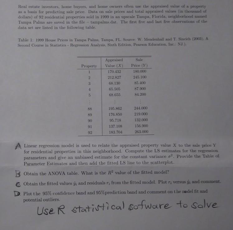
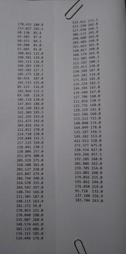
Real estate investors, home buyers, and home owners often use the appraised value of a property as a basis for predicting sale price. Data on sale prices and total appraised values in thousand of dollars) of 92 residential properties sold in 1999 in an upscale Tampa, Florida, neighborhood named Tampa Palms are saved in the file tampalms.dat. The first five and last five observations of the data set are listed in the following table. Table 1: 1999 House Prices in Tampa Palms. Tampa, FL. Source: W. Mendenhall and T. Sincich (2003). A Second Course in Statistics - Regression Analysis, Sixth Edition. Pearson Education, Inc., NJ.). Property 1 2 Appraised Value (X) 170.432 212.827 68.130 65.505 68.655 Sale Price (Y) 180.000 245.100 85.400 87.900 84.200 3 4 5 88 89 90 195.862 176.850 95.718 137.108 183.704 244.000 219.000 132.000 156.900 263.000 91 92 Linear regression model is used to relate the appraised property value X to the sale price Y for residential properties in this neighborhood. Compute the LS estimates for the regression parameters and give an unbiased estimate for the constant variance o?. Provide the Table of Parameter Estimates and then add the fitted LS line to the scatterplot. B. Obtain the ANOVA table. What is the R2 value of the fitted model? 3. Obtain the fitted values y, and residuals r; from the fitted model. Plot r; versus y, and comment. Plot the 95% confidence band and 95%prediction band and comment on the model fit and potential outliers. User statistical sofware to solve 171.1 12. 106.5 Jes. 172 205. 29, 30, 35. 365.0 120.01 0. 152.95 440 112.242 100. 225.613 220.0 15.14 187.0 169.282 214.8 121.832 185.0 172.432 la. 212.127 345,1 68.130 5.4 65,50587.8 68.655 4.2 64.930 25. 67 to 1. 100.0 125. les 91 124.6 102.523 126. 184.203 120.5 102.681 127.5 105.175 128.2 954 187.6 12.315 125. 119. 119 116.0 12.055 122.5 118.9 186.118 120. 1478855 1. 158.28 13.0 161.599 195.5 162. 195 193.0 153.475 192.0 2e3.826 2569 222.012 270.0 214.728 23.6 259.548 332.5 217.125 310.0 220.041 23.5 228.306 257.e 253.876 300. 285.529 275. 318.508 365. 202.127 258. 263.847 279.0 286.744 340.0 324.578 JS. 266.542 297.a 140.743 166.a 151.3es 187.0 148. 115 163.4 182.272 59.0 178.863 221. 270.84 299.a 235.087 2te. 348.574 445.0 302.133 486. 136.315 185.0 115.445 176.0 14,384 165.0 139.940 167. 127.705 164. 111.856 150.9 125.731 160.0 128.329 142.8 615.586 569. 572.523 715.0 140.04 170.0 164.849 178.0 125.187 156.5 149.282 153.0 422.911 528. 372.377 475.0 330.554 427.0 929.396 957.5 192.105 26e. 201.856 262.0 159.795 154.0 221.000 250. 179,056 215.2 195.862 244.0 176.858 219.0 95.718 132.0 137.10 156.9 183.704 263.0 Real estate investors, home buyers, and home owners often use the appraised value of a property as a basis for predicting sale price. Data on sale prices and total appraised values in thousand of dollars) of 92 residential properties sold in 1999 in an upscale Tampa, Florida, neighborhood named Tampa Palms are saved in the file tampalms.dat. The first five and last five observations of the data set are listed in the following table. Table 1: 1999 House Prices in Tampa Palms. Tampa, FL. Source: W. Mendenhall and T. Sincich (2003). A Second Course in Statistics - Regression Analysis, Sixth Edition. Pearson Education, Inc., NJ.). Property 1 2 Appraised Value (X) 170.432 212.827 68.130 65.505 68.655 Sale Price (Y) 180.000 245.100 85.400 87.900 84.200 3 4 5 88 89 90 195.862 176.850 95.718 137.108 183.704 244.000 219.000 132.000 156.900 263.000 91 92 Linear regression model is used to relate the appraised property value X to the sale price Y for residential properties in this neighborhood. Compute the LS estimates for the regression parameters and give an unbiased estimate for the constant variance o?. Provide the Table of Parameter Estimates and then add the fitted LS line to the scatterplot. B. Obtain the ANOVA table. What is the R2 value of the fitted model? 3. Obtain the fitted values y, and residuals r; from the fitted model. Plot r; versus y, and comment. Plot the 95% confidence band and 95%prediction band and comment on the model fit and potential outliers. User statistical sofware to solve 171.1 12. 106.5 Jes. 172 205. 29, 30, 35. 365.0 120.01 0. 152.95 440 112.242 100. 225.613 220.0 15.14 187.0 169.282 214.8 121.832 185.0 172.432 la. 212.127 345,1 68.130 5.4 65,50587.8 68.655 4.2 64.930 25. 67 to 1. 100.0 125. les 91 124.6 102.523 126. 184.203 120.5 102.681 127.5 105.175 128.2 954 187.6 12.315 125. 119. 119 116.0 12.055 122.5 118.9 186.118 120. 1478855 1. 158.28 13.0 161.599 195.5 162. 195 193.0 153.475 192.0 2e3.826 2569 222.012 270.0 214.728 23.6 259.548 332.5 217.125 310.0 220.041 23.5 228.306 257.e 253.876 300. 285.529 275. 318.508 365. 202.127 258. 263.847 279.0 286.744 340.0 324.578 JS. 266.542 297.a 140.743 166.a 151.3es 187.0 148. 115 163.4 182.272 59.0 178.863 221. 270.84 299.a 235.087 2te. 348.574 445.0 302.133 486. 136.315 185.0 115.445 176.0 14,384 165.0 139.940 167. 127.705 164. 111.856 150.9 125.731 160.0 128.329 142.8 615.586 569. 572.523 715.0 140.04 170.0 164.849 178.0 125.187 156.5 149.282 153.0 422.911 528. 372.377 475.0 330.554 427.0 929.396 957.5 192.105 26e. 201.856 262.0 159.795 154.0 221.000 250. 179,056 215.2 195.862 244.0 176.858 219.0 95.718 132.0 137.10 156.9 183.704 263.0