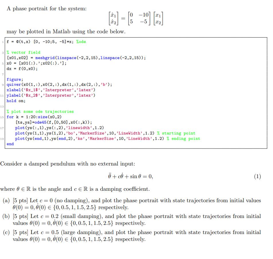
7 13 A phase portrait for the system: figure; 9quiver (x0 (1, :), x0 (2, :), dx (1, :), dx (2, :), 'b'); xlabel ('$x_1$', 'Interpreter', 'latex') 11 ylabel ('$x_2$', 'Interpreter', 'latex') hold on; 17 X1 % plot some ode trajectories 15 for k=1:20:size(x0,2) 19 may be plotted in Matlab using the code below. f = @(t, x) [0, -10;5, -5]*x; %ode 3% vector field. [x01,x02] = meshgrid (linspace (-2,2, 15), linspace (-2,2,15)); 5 X0 = [x01 (:).'; x02 (:).']; dx = f (0,x0); = 5 -10 -5 Consider a damped pendulum with no external input: [ts, ys] =ode45 (f, [0,50],x0(:,k)); plot (ys (:,1),ys (:,2), 'linewidth', 1.2) plot (ys (1,1),ys (1,2), 'bo', 'MarkerSize', 10, 'LineWidth',1.2) % starting point plot (ys (end, 1), ys (end, 2), 'ks', 'MarkerSize', 10, 'LineWidth', 1.2) % ending point end + c +sin 0 = 0, (1) where ER is the angle and c ER is a damping coefficient. (a) [5 pts] Let c = 0 (no damping), and plot the phase portrait with state trajectories from initial values 0(0) = 0,0(0) {0, 0.5, 1, 1.5, 2.5} respectively. (b) [5 pts] Let c = 0.2 (small damping), and plot the phase portrait with state trajectories from initial values 0(0) = 0,0(0) {0, 0.5, 1, 1.5, 2.5} respectively. (c) [5 pts] Let c = 0.5 (large damping), and plot the phase portrait with state trajectories from initial values 0(0) = 0, 0(0) {0,0.5, 1, 1.5, 2.5} respectively. 7 13 A phase portrait for the system: figure; 9quiver (x0 (1, :), x0 (2, :), dx (1, :), dx (2, :), 'b'); xlabel ('$x_1$', 'Interpreter', 'latex') 11 ylabel ('$x_2$', 'Interpreter', 'latex') hold on; 17 X1 % plot some ode trajectories 15 for k=1:20:size(x0,2) 19 may be plotted in Matlab using the code below. f = @(t, x) [0, -10;5, -5]*x; %ode 3% vector field. [x01,x02] = meshgrid (linspace (-2,2, 15), linspace (-2,2,15)); 5 X0 = [x01 (:).'; x02 (:).']; dx = f (0,x0); = 5 -10 -5 Consider a damped pendulum with no external input: [ts, ys] =ode45 (f, [0,50],x0(:,k)); plot (ys (:,1),ys (:,2), 'linewidth', 1.2) plot (ys (1,1),ys (1,2), 'bo', 'MarkerSize', 10, 'LineWidth',1.2) % starting point plot (ys (end, 1), ys (end, 2), 'ks', 'MarkerSize', 10, 'LineWidth', 1.2) % ending point end + c +sin 0 = 0, (1) where ER is the angle and c ER is a damping coefficient. (a) [5 pts] Let c = 0 (no damping), and plot the phase portrait with state trajectories from initial values 0(0) = 0,0(0) {0, 0.5, 1, 1.5, 2.5} respectively. (b) [5 pts] Let c = 0.2 (small damping), and plot the phase portrait with state trajectories from initial values 0(0) = 0,0(0) {0, 0.5, 1, 1.5, 2.5} respectively. (c) [5 pts] Let c = 0.5 (large damping), and plot the phase portrait with state trajectories from initial values 0(0) = 0, 0(0) {0,0.5, 1, 1.5, 2.5} respectively.