Using metrics to measure a software process

In this workshop you will learn how to calibrate your own personal software process by example. You’ll use Excel to convert existing data and create a line of best fit that you can use to evaluate the data. You’ll also learn how to test your model. Lastly, you’ll learn to compare your model against another model. Please show solution in Excel only step by step

Instructions

First, you need some data points (LOC, time). You have 10 points-keep one of these aside for the moment (i.e., don't use it in any calculations yet). Let’s keep the bottom point (291.0, 28.4) aside.

Code Size (LOC)	Time (Hours)
186.0	15.0
699.0	69.9
132.0	6.5
300.0	22.4
331.0	99.9
199.0	19.4
1890.0	198.7
788.0	38.8
1601.0	138.2
291.0	28.4

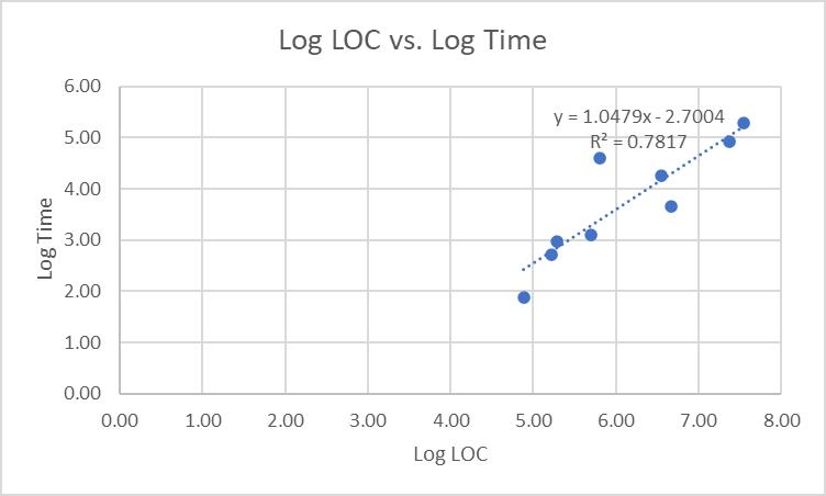
Second, we know that the relationship between those variables is not linear, therefore if we convert those values by taking the log of them, those log values would be linear i.e., if we plot log LOC vs. log time and do a line of best fit, we will get a straight line (of the form y = m*x +b). Take the logarithms of the LOC and time columns (except for the last row). Graph the results. They should look like this in Excel:

In R, the output looks a little different, but notice that the results are the same:

Coefficients:

Estimate Std. Error t value Pr(>|t|)

(Intercept) -2.7004 1.2941 -2.087 0.07534 .

logLOC 1.0479 0.2093 5.007 0.00155 **

---

Signif. codes: 0 ‘***’ 0.001 ‘**’ 0.01 ‘*’ 0.05 ‘.’ 0.1 ‘ ’ 1

Residual standard error: 0.5688 on 7 degrees of freedom

Multiple R-squared: 0.7817, Adjusted R-squared: 0.7506

F-statistic: 25.07 on 1 and 7 DF, p-value: 0.001553

Now we have a model that can predict time, given lines of code.

Having created a line of best fit (in Excel or other tool of your choice) you can now talk about the constants and what they mean, how good your line is (the Correlation Coefficient and Coefficient of Determination) and the effect of any outliers.

Notice that r² (the Coefficient of Determination) is 0.7817, so approximately 78% of Time is explained by LOC. What about the other 22%? The r value (the Correlation Coefficient, the square root of the Coefficient of Determination) is 0.88-pretty good, but what about the missing 22%? Is the model missing a variable or does it just need fine-tuning?

Notice that one of the points is much further from the line of best fit than the others. We call this an outlier – a data point that looks significant different from the other points in our set. A common way to determine an outlier is to calculate the standardised residuals and see if any are greater than some cutoff value (often 3, sometimes 2, depending on the level of rigour required). The residual is a measure of the strength of the difference between observed and expected values-in our case, that means the vertical difference between the line of best fit and the actual data value. if the data are normally distributed, 95% of the data should be within two standard deviations from the mean, so we choose 2 as our cutoff value to determine an outlier.

Both Excel and R can calculate and display the standardised residuals. In R, the residuals look like this:

1 2 3 4 5 6 7

-0.1347387 0.1587607 -1.1587044 -0.3168153 2.3004551 0.2336835 0.1937862

8 9

-1.2036914 -0.2204413

We see that one value has an absolute value greater than 2.

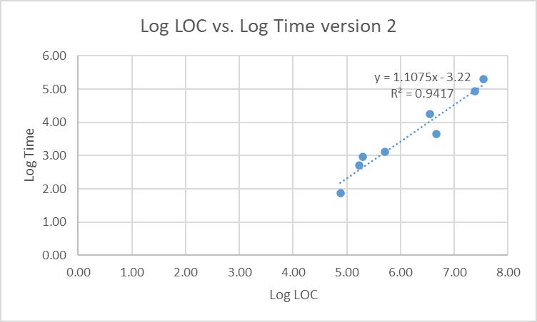
Remove that point from the model and recalculate. Do the r² and r values improve? The adjusted model should look like this in Excel:

Or in R:

Coefficients:

Estimate Std. Error t value Pr(>|t|)

(Intercept) -3.2200 0.7009 -4.594 0.00371 **

logLOC 1.1075 0.1125 9.843 6.34e-05 ***

---

Signif. codes: 0 ‘***’ 0.001 ‘**’ 0.01 ‘*’ 0.05 ‘.’ 0.1 ‘ ’ 1

Residual standard error: 0.3035 on 6 degrees of freedom

Multiple R-squared: 0.9417, Adjusted R-squared: 0.932

F-statistic: 96.89 on 1 and 6 DF, p-value: 6.338e-05

Notice that r² has improved at 0.9417, so approximately 94% of Time is explained by LOC. The r value is now 0.971 – very good.

You also need to test your model. We can do this in two ways, internally and externally. First, the internal test. There are several ways to do this. One is to select a value that is on (or very close to) the line of best fit. Let’s choose (5.70, 3.11).

The model says y = 1.1075x – 3.22

Substituting in we get y = 1.1075*5.70 - 3.22

Or y = 3.09, which compares favourably with the actual value (3.11). The difference might be due to calculating to 2 decimal places (if we use the values from R, we get 3.0969 or 3.10 to 2dp). This tells us that our model performs correct calculations.

Now, the external test. Remember the point you kept aside at the start? For this point, you know the answer. What does your predictive model say? Is it any good?

The model says y = 1.1075x – 3.22

Substituting in we get y = 1.1075*5.67 - 3.22

Or y = 3.059525, which compares favourably with the actual value (3.35).

Remember, these are the logarithms of the values, so if you want to see LOC, and not log(LOC), you now need to reverse the logarithm by taking the antilog of 3.059525 (which gives LOC = 21.32). It is not perfect (as 21.32 ≠ 28.4). Why do think this might be so? What could affect the variables in your model?

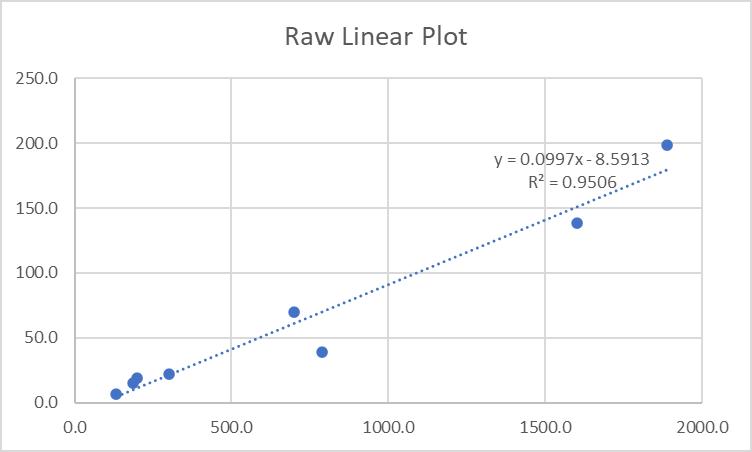
Finally, you want to examine the linearity of your raw data. You know it's not linear, but what if you plotted it as if it were linear? Do you get a better result than your log-log model? Why might that be so? Let’s try that with the raw data (without the outlier point) in Excel:

In R:

Coefficients:

Estimate Std. Error t value Pr(>|t|)

(Intercept) -8.591330 8.935453 -0.961 0.373

Code.Size..LOC. 0.099677 0.009274 10.748 3.83e-05 ***

---

Signif. codes: 0 ‘***’ 0.001 ‘**’ 0.01 ‘*’ 0.05 ‘.’ 0.1 ‘ ’ 1

Residual standard error: 16.66 on 6 degrees of freedom

Multiple R-squared: 0.9506, Adjusted R-squared: 0.9424

F-statistic: 115.5 on 1 and 6 DF, p-value: 3.833e-05

Notice that r² has improved marginally to 0.9506, so approximately 95% of Time is explained by LOC. The r value is now 0.975-another slight improvement. The previous model is correct mathematically, so that is the one we should use.

What you have done is built a calibrated estimation model, which is what you would do in practice.

Show solution in Excel demonstrate visually please step by step. 

Log Time 6.00 5.00 Log LOC vs. Log Time y 1.0479x-2.7004 R = 0.7817 4.00 3.00 2.00 1.00 0.00 0.00 1.00 2.00 3.00 4.00 5.00 6.00 7.00 8.00 Log LOC