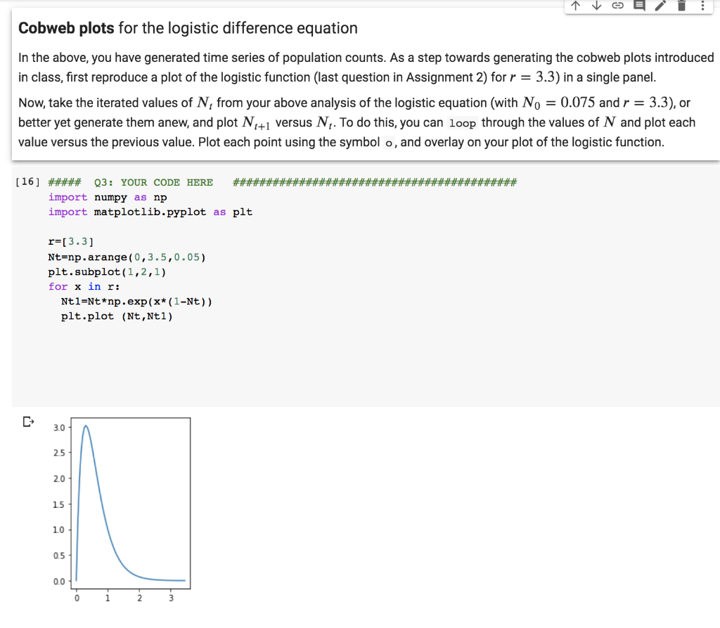
(using Python) ive reproduced the logistic plot in a single panel. use my answer in the logistic difference equation to answer the cobweb plots question

This is part 2 of the question:

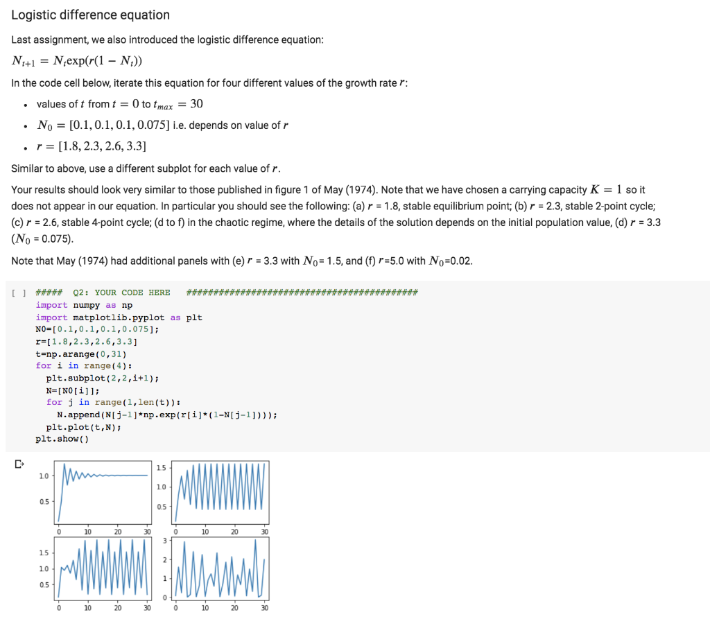
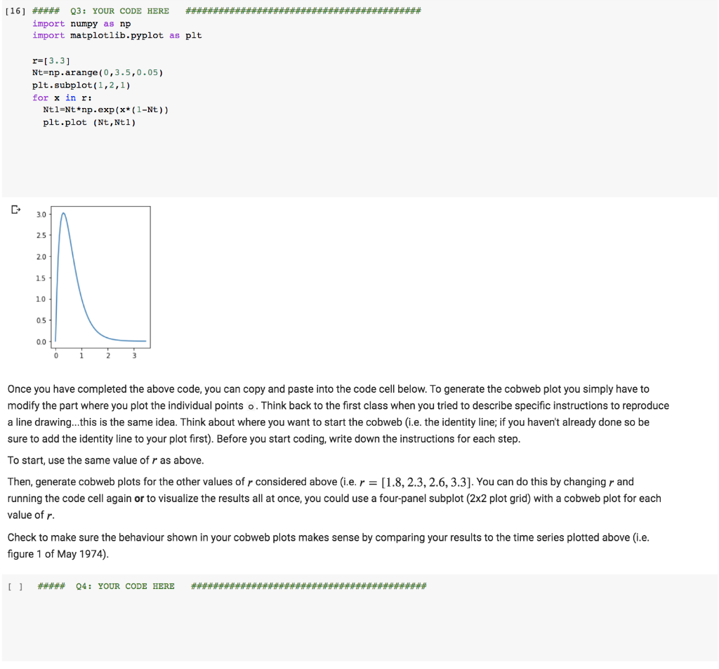
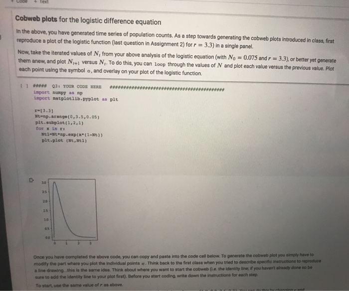
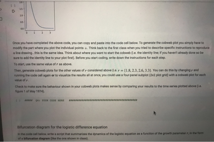
Cobweb plots for the logistic difference equation In the above, you have generated time series of population counts. As a step towards generating the cobweb plots introduced in class, first reproduce a plot of the logistic function (last question in Assignment 2) for r = 3.3) in a single panel. Now, take the iterated values of N, from your above analysis of the logistic equation (with No = 0.075 andr = 3.3), or better yet generate them anew, and plot N1+1 versus N,. To do this, you can loop through the values of N and plot each value versus the previous value. Plot each point using the symbol o, and overlay on your plot of the logistic function. [16] ##### Q3: YOUR CODE HERE ### ##2# import numpy as np import matplotlib.pyplot as plt r=[3.3] Nt=np.arange (0,3.5,0.05) plt.subplot (1,2,1) for x in r: Ntl=Nt*np.exp(x* (1-Nt)) plt.plot (Nt,Ntl) 3.0 25 2.0 15 10 0.5 0.0 Logistic difference equation Last assignment, we also introduced the logistic difference equation: N+1 = N,exp(r(1 N;)) In the code cell below, iterate this equation for four different values of the growth rate r: values of t from t = 0 to t max = 30 No = [0.1,0.1, 0.1, 0.075] i.e. depends on value of r r = [1.8, 2.3, 2.6, 3.3] Similar to above, use a different subplot for each value of r. Your results should look very similar to those published in figure 1 of May (1974). Note that we have chosen a carrying capacity K = 1 so it does not appear in our equation. In particular you should see the following: (a) r = 1.8, stable equilibrium point; (b) r = 2.3, stable 2-point cycle; (c) r = 2.6, stable 4-point cycle; (d to f) in the chaotic regime, where the details of the solution depends on the initial population value, (d) r = 3.3 (No = 0.075). Note that May (1974) had additional panels with (e) r = 3.3 with No= 1.5, and (f) r=5.0 with No=0.02. [] ##### Q2: YOUR CODE HERE ##### ####* import numpy as np import matplotlib.pyplot as plt NO=[0.1,0.1,0.1,0.075]; r=[1.8,2.3,2.6,3.3] t=np.arange (0,31) for i in range(4): plt.subplot(2,2,i+1); N=[NO[i]]; for j in range (1,len(t)) : N.append (N[j-l]*np.exp(r[i]* (1-N[j-1]))); plt.plot(t,N); plt.show () 15 10 10 0.5 0.5 10 10 20 30 15 10 0.5 10 30 ##******** [16] ##### Q3: YOUR CODE HERE #####*****## import numpy as np import matplotlib.pyplot as plt r=[3.3] Nt=np.arange (0,3.5,0.05) plt.subplot(1,2,1) for x in r: Ntl=Nt*np.exp (x* (1-Nt)) plt.plot (Nt,Ntl) 30 2.5 2.0 15 10 0.5 0.0 Once you have completed the above code, you can copy and paste into the code cell below. To generate the cobweb plot you simply have to modify the part where you plot the individual points o. Think back to the first class when you tried to describe specific instructions to reproduce a line drawing.this is the same idea. Think about where you want to start the cobweb (i.e. the identity line; if you haven't already done so be sure to add the identity line to your plot first). Before you start coding, write down the instructions for each step. To start, use the same value of r as above. Then, generate cobweb plots for the other values of r considered above (i.e. r = [1.8, 2.3, 2.6, 3.3]. You can do this by changing r and running the code cell again or to visualize the results all at once, you could use a four-panel subplot (2x2 plot grid) with a cobweb plot for each value of r. Check to make sure the behaviour shown in your cobweb plots makes sense by comparing your results to the time series plotted above (i.e. figure 1 of May 1974). ##### Q4: YOUR CODE HERE + Text Cobweb plots for the logistic difference equation In the above, you have generated time series of population counts. As a step towards generating the cobweb plots introduced in class, first reproduce a plot of the logistic function (last question in Assignment 2) for r = 3.3) in a single panel. Now, take the iterated values of N, from your above analysis of the logistic equation (with No = 0.075 and r= 3.3), or better yet generate them anew, and plot N+1 versus N. To do this, you can loop through the values of N and plot each value versus the previous value. Plot each point using the symbol o, and overlay on your plot of the logistic function. I Q3: YOUR CODE HERE import numpy as np import matplotlib.pyplot as plt r-[3.3] Nt-np.arange(0,3.5,0.05) plt.subplot (1,2,1) for x in r! Ntl-Ntnp.exp(x(1-Nt)) plt.plot (Nt, Nt1) 30 25 20 15 10 00 Once you have completed the above code, you can copy and paste into the code cell below. To generate the cobweb plot you simply have to modify the part where you plot the individual points e. Think back to the first class when you tried to describe specific instructions to reproduce a line drawing. this is the same idea. Think about where you want to start the cobweb (le. the identity line, if you haven't already done so be sure to add the identity line to your plot first). Before you start coding, write down the instructions for each step. To start, use the same value of r as above. thistchannninnand 20 15 10 05 00 Once you have completed the above code, you can copy and paste into the code cell below. To generate the cobweb plot you simply have to modify the part where you plot the individual points o. Think back to the first class when you tried to describe specific instructions to reproduce a line drawing. this is the same idea. Think about where you want to start the cobweb (i.e. the identity line; if you haven't already done so be sure to add the identity line to your plot first). Before you start coding, write down the instructions for each step. To start, use the same value of r as above. Then, generate cobweb plots for the other values of r considered above (1.e. r = [1.8, 2.3, 2.6, 3.3). You can do this by changing r and running the code cell again or to visualize the results all at once, you could use a four-panel subplot (2x2 plot grid) with a cobweb plot for each value of r. Check to make sure the behaviour shown in your cobweb plots makes sense by comparing your results to the time series plotted above (L.e. figure 1 of May 1974). 041 YOUR CODE HERE 11 Bifurcation diagram for the logistic difference equation In the code cell below, write a script that summarizes the dynamics of the logistic equation as a function of the growth parameter r, in the form of a bifurcation diagram (like the one shown in class). Cobweb plots for the logistic difference equation In the above, you have generated time series of population counts. As a step towards generating the cobweb plots introduced in class, first reproduce a plot of the logistic function (last question in Assignment 2) for r = 3.3) in a single panel. Now, take the iterated values of N, from your above analysis of the logistic equation (with No = 0.075 andr = 3.3), or better yet generate them anew, and plot N1+1 versus N,. To do this, you can loop through the values of N and plot each value versus the previous value. Plot each point using the symbol o, and overlay on your plot of the logistic function. [16] ##### Q3: YOUR CODE HERE ### ##2# import numpy as np import matplotlib.pyplot as plt r=[3.3] Nt=np.arange (0,3.5,0.05) plt.subplot (1,2,1) for x in r: Ntl=Nt*np.exp(x* (1-Nt)) plt.plot (Nt,Ntl) 3.0 25 2.0 15 10 0.5 0.0 Logistic difference equation Last assignment, we also introduced the logistic difference equation: N+1 = N,exp(r(1 N;)) In the code cell below, iterate this equation for four different values of the growth rate r: values of t from t = 0 to t max = 30 No = [0.1,0.1, 0.1, 0.075] i.e. depends on value of r r = [1.8, 2.3, 2.6, 3.3] Similar to above, use a different subplot for each value of r. Your results should look very similar to those published in figure 1 of May (1974). Note that we have chosen a carrying capacity K = 1 so it does not appear in our equation. In particular you should see the following: (a) r = 1.8, stable equilibrium point; (b) r = 2.3, stable 2-point cycle; (c) r = 2.6, stable 4-point cycle; (d to f) in the chaotic regime, where the details of the solution depends on the initial population value, (d) r = 3.3 (No = 0.075). Note that May (1974) had additional panels with (e) r = 3.3 with No= 1.5, and (f) r=5.0 with No=0.02. [] ##### Q2: YOUR CODE HERE ##### ####* import numpy as np import matplotlib.pyplot as plt NO=[0.1,0.1,0.1,0.075]; r=[1.8,2.3,2.6,3.3] t=np.arange (0,31) for i in range(4): plt.subplot(2,2,i+1); N=[NO[i]]; for j in range (1,len(t)) : N.append (N[j-l]*np.exp(r[i]* (1-N[j-1]))); plt.plot(t,N); plt.show () 15 10 10 0.5 0.5 10 10 20 30 15 10 0.5 10 30 ##******** [16] ##### Q3: YOUR CODE HERE #####*****## import numpy as np import matplotlib.pyplot as plt r=[3.3] Nt=np.arange (0,3.5,0.05) plt.subplot(1,2,1) for x in r: Ntl=Nt*np.exp (x* (1-Nt)) plt.plot (Nt,Ntl) 30 2.5 2.0 15 10 0.5 0.0 Once you have completed the above code, you can copy and paste into the code cell below. To generate the cobweb plot you simply have to modify the part where you plot the individual points o. Think back to the first class when you tried to describe specific instructions to reproduce a line drawing.this is the same idea. Think about where you want to start the cobweb (i.e. the identity line; if you haven't already done so be sure to add the identity line to your plot first). Before you start coding, write down the instructions for each step. To start, use the same value of r as above. Then, generate cobweb plots for the other values of r considered above (i.e. r = [1.8, 2.3, 2.6, 3.3]. You can do this by changing r and running the code cell again or to visualize the results all at once, you could use a four-panel subplot (2x2 plot grid) with a cobweb plot for each value of r. Check to make sure the behaviour shown in your cobweb plots makes sense by comparing your results to the time series plotted above (i.e. figure 1 of May 1974). ##### Q4: YOUR CODE HERE + Text Cobweb plots for the logistic difference equation In the above, you have generated time series of population counts. As a step towards generating the cobweb plots introduced in class, first reproduce a plot of the logistic function (last question in Assignment 2) for r = 3.3) in a single panel. Now, take the iterated values of N, from your above analysis of the logistic equation (with No = 0.075 and r= 3.3), or better yet generate them anew, and plot N+1 versus N. To do this, you can loop through the values of N and plot each value versus the previous value. Plot each point using the symbol o, and overlay on your plot of the logistic function. I Q3: YOUR CODE HERE import numpy as np import matplotlib.pyplot as plt r-[3.3] Nt-np.arange(0,3.5,0.05) plt.subplot (1,2,1) for x in r! Ntl-Ntnp.exp(x(1-Nt)) plt.plot (Nt, Nt1) 30 25 20 15 10 00 Once you have completed the above code, you can copy and paste into the code cell below. To generate the cobweb plot you simply have to modify the part where you plot the individual points e. Think back to the first class when you tried to describe specific instructions to reproduce a line drawing. this is the same idea. Think about where you want to start the cobweb (le. the identity line, if you haven't already done so be sure to add the identity line to your plot first). Before you start coding, write down the instructions for each step. To start, use the same value of r as above. thistchannninnand 20 15 10 05 00 Once you have completed the above code, you can copy and paste into the code cell below. To generate the cobweb plot you simply have to modify the part where you plot the individual points o. Think back to the first class when you tried to describe specific instructions to reproduce a line drawing. this is the same idea. Think about where you want to start the cobweb (i.e. the identity line; if you haven't already done so be sure to add the identity line to your plot first). Before you start coding, write down the instructions for each step. To start, use the same value of r as above. Then, generate cobweb plots for the other values of r considered above (1.e. r = [1.8, 2.3, 2.6, 3.3). You can do this by changing r and running the code cell again or to visualize the results all at once, you could use a four-panel subplot (2x2 plot grid) with a cobweb plot for each value of r. Check to make sure the behaviour shown in your cobweb plots makes sense by comparing your results to the time series plotted above (L.e. figure 1 of May 1974). 041 YOUR CODE HERE 11 Bifurcation diagram for the logistic difference equation In the code cell below, write a script that summarizes the dynamics of the logistic equation as a function of the growth parameter r, in the form of a bifurcation diagram (like the one shown in class)