Using Table 6-2 as a guide, compare and contrast predictive and prescriptive analytics. How might these be used in an audit? Or a continuous audit?

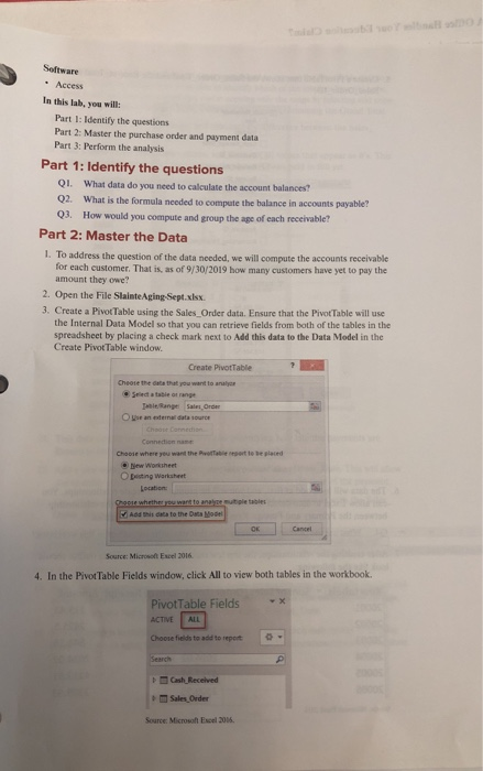
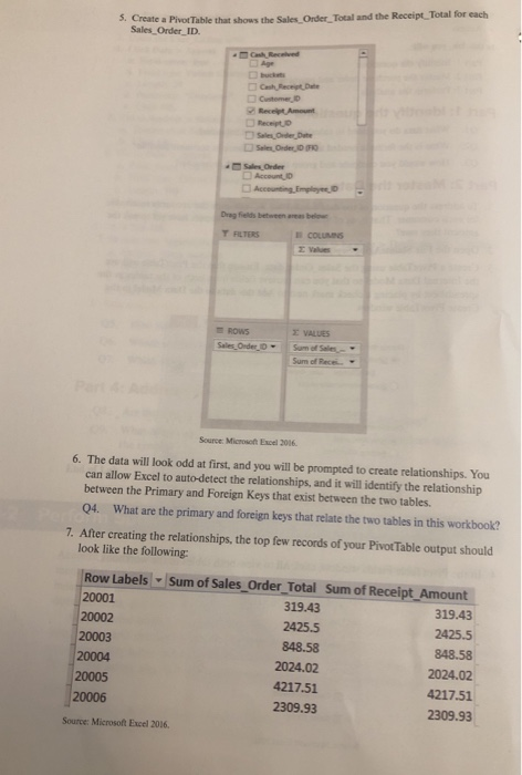
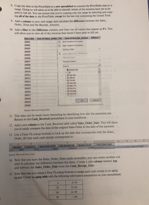
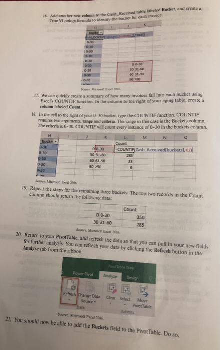
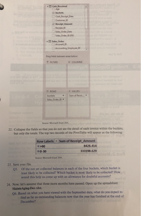
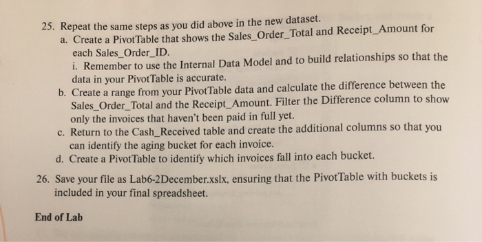
6-2 Perform Substantive Tests of Account Balances Account balances do not exist in databases. Rather, they are the combination of data ele- ments that are added together to come up with a total through queries and formulas. The balance for accounts payable, for example is the combination of invoices received, cash disbursements, and debit memos As an internal auditor, you have been tasked with validating the balance in accounts receiv- able. Your audit manager has given you a list of receivables for comparison. Additionally company policy states that accounts receivables should be collected within 60 days of the sale. To test this policy, you have been asked to perform an aging of outstanding accounts Techniques Use Excel tools to calculate account balances Use Excel tools to group accounts by age mi olb Software Access In this lab. vou will: Part I: Identify the questions Part 2: Master the purchase order and payment datar Part 3: Perform the analysis. Part 1: Identify the questions QI. What data do you need to calculate the account balances? Q2. What is the formula needed to compute the balance in accounts payable? Q3. How would you compute and group the age of each receivable? Part 2: Master the Data 1. To address the question of the data needed, we will compute the accounts receivable for each customer. That is, as of 9/30/2019 how many customers have yet to pay the amount they owe? 2. Open the File SlainteAging-Sept.xlsx 3. Create a PivotTable using the Sales Order data. Ensure that the PivotTable will use the Internal Data Model so that you can retrieve fields from both of the tables in the spreadsheet by placing a check mark next to Add this data to the Data Model in the Create PivotTable window. Create PivotTable Cheose the data that you want to analyce Select a table ot range esleRange Sales Order Oge an edemal data sources Choose Connedion Connection name Choose where veu want the Pvotfable report to be placed .New Worksheet Opesting Warksheet Location Choose whether you want to analpe mutiple tables Add this data to the Data Mo0e Cancel Source: Microsoft Excel 2016 4. In the PivotTable Fields window, click All to view both tables in the workbook. PivotTable Fields ACTIVE ALL Choose fields to add to report Search Cash Received Sales Order Source: Microsoft Escel 2016 5. Create a PivotTable that shows the Sales Order Total and the Receipt Total for each Sales Order ID aCash Recelved Age bucksts Cash Recipt Dee Customer D Recelpt Amount Receipt D Seles Order Date Seles Order,ID (F Sales Order Account ID Accounting Empleyee,D Drag fields between areas below COLUMINS T RLTERS E Values E VALUES ROWS Sales Order D Sum of Sales Sum of Rece Source: Microsofh Excel 2016. 6. The data will look odd at first, and you will be prompted to create relationships. You can allow Excel to auto-detect the relationships, and it will identify the relationship between the Primary and Foreign Keys that exist between the two tables 04 What are the primary and foreign keys that relate the two tables in this workbook? Perfo 7. After creating the relationships, the top few records of your Pivot Table output should look like the following Row Labels Sum of Sales_Order_Total Sum of Receipt_Amount 20001 319.43 319.43 20002 2425.5 2425.5 20003 848.58 848.58 20004 2024.02 2024.02 20005 4217.51 4217.51 20006 2309.93 2309.93 Source: Microsoft Excel 2016 . Copy the data in the PivotTable to a new spreadsheet to convert the PivotTable data to a range. Doing so will allow us to be able to identify which of the invoices have yet to be paid in full yet. You can ensure that you're copying only the range by selecting and copy- ing all of the data in the PivotTable, except for the last row containing the Grand Total. 9. Add a column to your new range, and calculate the difference between the Sales Order Total and the Receipt Amount. 10. Add a filter to the Difference column, and filter out all values that appear as 0's. This will allow you to view all of the invoices that haven't been paid in full yet. Row Labe Sum of Sales Order TotSum of Recelpt AmourDiffere Sot Smallest to Largest 20001 20002 lSot Largest to Smallest 20003 Sot by Color 20004 Der Fiter From Dference" 20005 Fiter by Color 20006 20007 Number Eilters 20008 Search 20009 Select Al 20010 202.524 268.05 20011 20012 27699 284.046 208.774 304.514 309.86 20013 20014 20015 20016 340.459 20017 20018 OK Cancel 20019 20020 Source: Microson Excel 2016 11. This data can be made more interesting by identifying how late the payments are. Return to the Cash_Received spreadsheet in your workbook 12. Add a new column to the Cash Received table called Sales Order Date. This will allow you to easily compare the date of the original Sales Order to the date of the payment. 13. Use a False VLookup formula to look up the date that corresponds with the Sales Order_ID that each cash receipt corresponds to. N M Receipt Amourw 63. Sales Order Date Sales Order ID (F Cash Receipt Dat- 20001 Sales Onder 2,FALSE Customer Receipt - VLOOKUPLOSales Order o 1/10/2035 2024 10001 Source: Microsoft Excel 2016. 14. Now that you have the Sales Order Date easily accessible, you can create another col- umn to calculate the difference between the dates. Create a new column labeled Age, and subtract the Sales Order Date from the Cash Receipt Date. 15. Your next step is to create a True VLookup formula to assign each cash receipt to an aging bucket. Create an aging table with the following information somewhere on your spreadsheet: 0-30 0 31-60 30 61-90 60 >90 90 16. Add another new eolumn to the Cash Received table labeled Bucket, and create a True VLookup formula to identify the bucket for each invoice. VLOOKUPesgelbucket 2,TRUE P-30 i0-30 bucke :0-30 i0-30 0-30 o 0-30 o-30 30 31-60 s0 61-90 .0-30 iD-30 s090 .D-30 Soune Microwt Excel 206 17. We can quickly create a summary of how many invoices fall into each bucket using Excel's COUNTIF fanction. In the column to the right of your aging table, create a column labeled Count 18. In the cell to the right of your requires two arguments, range and criteria. The range in this case is the Buckets column. The criteria is 0-30. COUNTIF will count every instance of 0-30 in the buckets column. ket, type the COUNTIF function. COUNTIF N M K L bucke Count COUNTIF(Cash Received[buckets], K2) 285 ol0-30 30 31-50 0-30 0-30 0-30 0-30 0-30 60 61-90 33 9090 Source: Microsot Excel 2016 19. Repeat the steps for the remaining three buckets. The top two records in the Count column should return the following data Count 0 0-30 350 30 31-60 285 Source: Microsoft Excel 2006 20. Return to your PivotTable, and refresh the data so that you can pull in your new fields for further analysis. You can refresh your data by clicking the Refresh button in the Analyze tab from the ribbon. PTeble Tools Power Pvot Analyce Design Refresh Change Data Source Clear Select Move PivotTable Data Actions Source: Microsoft Excel 2016 21. You should now be able to add the Buckets field to the Pivot Table. Do so Cash Received Age buckets Cash Receipt Date Customer ID Receipt Amount Receipt ID Sales Order Date Sales Order ID (F Sales Order Account ID Accounting Empleye, D Drag fields between areas below E COLUMNS T FLTERS mamys9tlqua pnibnia E VALUES ROWS tob 6.4 Cor Hy Sum of Recei. buckets Sales Order ID Source: Microsoft Excel 2016 22. Collapse the fields so that you do not see the detail of each invoice within the buckets. but only the totals. The top two records of the PivotTable will appear as the following Sum of Receipt Amount Row Labels 8428.414 >90 333198.629 80-30 Source Microsoft Excel 2016 23. Save your file. Of the not yet collected balances in each of the four buckets, which bucket is QS. least likely to be collected? Which bucket is most likely to be collected? wouid this help us come up with an allowance for doubtful accounts? How 24. Now, let's assume that three more months have passed. Open up the spreadsheet SlainteAging-Dec.xlsx. 06, Based on what you have viewed with the September data, what do you expect to find as far as outstanding balances now that the year has finished at the end of December? 25. Repeat the same steps as you did above in the new dataset. Create a PivotTable that shows the Sales_Order_Total and Receipt_Amount for each Sales_Order_ID i. Remember to use the Internal Data Model and to build relationships so that the data in your PivotTable is accurate b. Create a range from your PivotTable data and calculate the difference between the Sales_Order_Total and the Receipt_Amount. Filter the Difference column to show only the invoices that haven't been paid in full yet. c. Return to the Cash_Received table and create the additional columns so that you can identify the aging bucket for each invoice. d. Create a PivotTable to identify which invoices fall into each bucket. a. 26. Save your file as Lab6-2December.xslx, ensuring that the PivotTable with buckets is included in your final spreadsheet. End of Lab