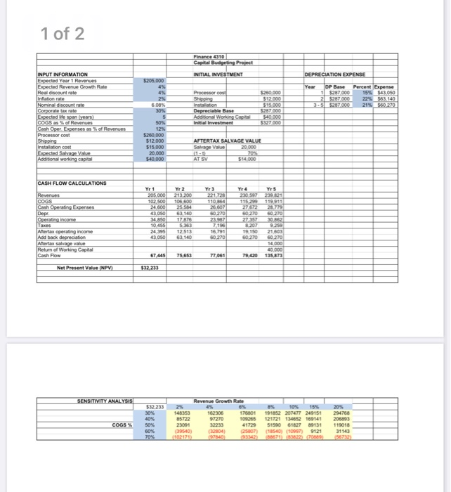
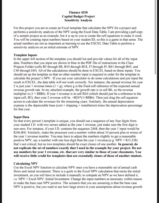
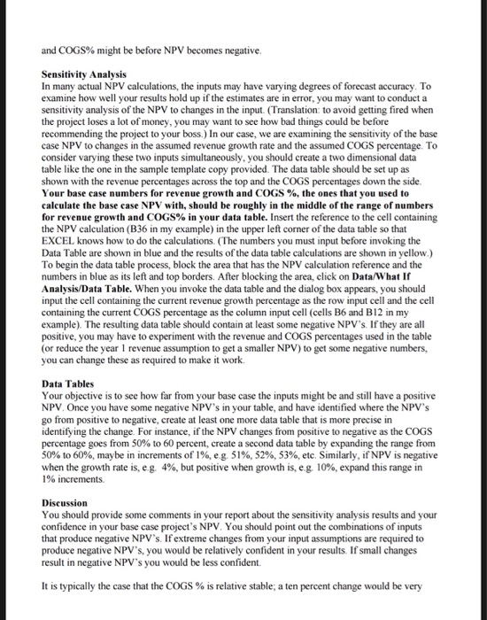
Using the attached instructions, perform a sensitivity analysis of Net Present Value (NPV) using the Excel Data Table. Submit the required Excel spreadsheets and your analysis using the Assignment Tool. 1 of 2 Finance 43101 Capital Budgeting Project INPUT INFORMATION Expected Year 1 Revenues INITIAL INVESTMENT DEPRECIATION EXPENSE 5205 000 Year DP Base $287.000 21 $287.000 3. $287.000 Percent Expense 15% $43 050 22% 563.140 21% 560270 Inflation rate 608% Depreciable Base AFTERTAX SALVAGE VALUE Salvage Value $12,000 $15.000 20.000 $40,000 Espected Salvage Val Additional working capital CASH FLOW CALCULATIONS Y5 205 000 1027500 24600 Yr3 221728 110 864 Cash Operating Expenses Yr 2 213 200 106.600 25584 63,140 17875 28.77 20 10 455 24 395 43.050 23. 987 7.196 16.791 60.270 19.150 63 140 21.503 60270 Add back depreciation Attertax salvage value Return of Working Capital 5000 67.445 75,653 7 70511 Net Present Value (NPV) SENSITIVITY ANALYSIS S8233 176801 191852 20147 249151 COGS 4177295159061827 99131119018 2 ST SAD 099) 91213 1143 Finance 4310 Capital Budget Project Sensitivity Analysis For this project you are to create an Excel template that calculates the NPV for a project and performs a sensitivity analysis of the NPV using the Excel Data Table. I am providing a pdf copy of a sample project as an example, but it is up to you to create the cell equations to make it work. You will be creating input numbers based on your student ID, so this is a game in that sense. The actual numbers are not as important as learning to use the EXCEL Data Table to perform a sensitivity analysis on an initial estimate of NPV. Template Inputs In the upper left section of the template you should list and provide values for all of the input data. Numbers that you input are shown in blue in the PDF file of instructions in the Class Projects Folder (cells B5 through B8, B10 through B18, J7 through J9, B41 through B45, and C40 through 140). All of the calculations should be done in EXCEL based on these inputs. You should set up the template so that no other number input is required in order for the template to calculate the project's NPV. If you use your calculator to do some calculations and just input the result in EXCEL, the data table will not work correctly. For instance, the annual revenue for year 2 is just year I revenue times (1 + g), where g is the fixed cell reference of the expected annual revenue growth rate. In my attached example, the growth rate is in cell B6, so the revenue multiplier is (1 + $B$6). If year I revenue is in cell B24 (which should just be a reference to the input cell, B5), then year 2 revenue will be -B24*(1+$B$6). Then just drag the cell equation across to calculate the revenues for the remaining years. Similarly, the annual depreciation expense is the depreciable base (cost + shipping + installation) times the depreciation percentage for that year Input Data So that every person's template is unique, you should use a sequence of any four digits from your student ID with two zeroes added as the year 1 revenue, just make sure the first digit is non-zero. For instance, if your ID contains the sequence 2468, then the year 1 input would be $246,800. Similarly, make the processor cost a number within about 10 percent plus or minus of the year I revenue number. You may have to adjust the numbers slightly to get a reasonable positive NPV, say a number with one less digit than the year I revenue,(e.g. NPV - $15,338) that's not critical, but no two templates should be exact clones of one another. In general, do not replicate the set of numbers exactly that I used in the example for your project. Do not use numbers for year I revenue, etc. that are very similar to those of your classmates. You will receive little credit for templates that are essentially clones of those of another student. Calculating NPV Use the Excel NPV function to calculate NPV once you have a reasonable set of annual cash flows and initial investment. There is a quirk in the Excel NPV calculation that omits the initial investment, so you will have to include it manually to compute an NPV as we have defined it, ie NPV-Excel NPV-Initial Investment Change the input numbers as necessary within reason to make the base case NPV positive. The scenario that you are assuming is that the base case NPV is positive, but you want to see how large errors in your assumptions about revenue growth and COGS% might be before NPV becomes negative. Sensitivity Analysis In many actual NPV calculations, the inputs may have varying degrees of forecast accuracy. To how well your results hold up if the estimates are in error, you may want to conduct a sensitivity analysis of the NPV to changes in the input. (Translation: to avoid getting fired when the project loses a lot of money, you may want to see how bad things could be before recommending the project to your boss.) In our case, we are examining the sensitivity of the base case NPV to changes in the assumed revenue growth rate and the assumed COGS percentage. To consider varying these two inputs simultaneously, you should create a two dimensional data table like the one in the sample template copy provided. The data table should be set up as shown with the revenue percentages across the top and the COGS percentages down the side Your base case numbers for revenue growth and COGS %, the ones that you used to calculate the base case NPV with, should be roughly in the middle of the range of numbers for revenue growth and COGS% in your data table. Insert the reference to the cell containing the NPV calculation (B36 in my example) in the upper left corner of the data table so that EXCEL knows how to do the calculations. (The numbers you must input before invoking the Data Table are shown in blue and the results of the data table calculations are shown in yellow.) To begin the data table process, block the area that has the NPV calculation reference and the numbers in blue as its left and top borders. After blocking the area, click on Data/What If Analysis/Data Table. When you invoke the data table and the dialog box appears, you should input the cell containing the current revenue growth percentage as the row input cell and the cell containing the current COGS percentage as the column input cell (cells B6 and B12 in my example). The resulting data table should contain at least some negative NPV's. If they are all positive, you may have to experiment with the revenue and COGS percentages used in the table (or reduce the year I revenue assumption to get a smaller NPV) to get some negative numbers, you can change these as required to make it work Data Tables Your objective is to see how far from your base case the inputs might be and still have a positive NPV. Once you have some negative NPV's in your table, and have identified where the NPV'S go from positive to negative, create at least one more data table that is more precise in identifying the change. For instance, if the NPV changes from positive to negative as the COGS percentage goes from 50% to 60 percent, create a second data table by expanding the range from 50% to 60%, maybe in increments of 1%, eg 51%, 52%, 53%, etc. Similarly, if NPV is negative when the growth rate is, eg 4%, but positive when growth is, eg 10%, expand this range in 1% increments Discussion You should provide some comments in your report about the sensitivity analysis results and your confidence in your base case project's NPV. You should point out the combinations of inputs that produce negative NPV's. If extreme changes from your input assumptions are required to produce negative NPV's, you would be relatively confident in your results. If small changes result in negative NPV's you would be less confident. It is typically the case that the COGS % is relative stable, a ten percent change would be very significant. So if the data table shows that COGS must increase by more than ten percent from your original assumption before negative NPV's occur, you would feel very confident in your original calculation. On the other hand, if only a four percent increase in COGS would result in a negative NPV, you would be much less confident in your original estimate. Format You can submit everything in Excel for this project. Just include your name, the class and section, and the due date at the top of the template. You can also put your discussion in the Excel template. I need to see the Excel version so that I can see your cell equations, so don't convert it to pdf or word. Due Date: Stated in the syllabus. Use the assignment tool to submit the project. Since all the required input is in Excel format, there will be no need to scan to pdf. Caveat Obviously, in a real project you would not be able to adjust the input numbers to get the answer you want, but since we are most interested in learning to conduct a sensitivity analysis and interpret its results, we are taking some unusual liberties with our inputs. Using the attached instructions, perform a sensitivity analysis of Net Present Value (NPV) using the Excel Data Table. Submit the required Excel spreadsheets and your analysis using the Assignment Tool. 1 of 2 Finance 43101 Capital Budgeting Project INPUT INFORMATION Expected Year 1 Revenues INITIAL INVESTMENT DEPRECIATION EXPENSE 5205 000 Year DP Base $287.000 21 $287.000 3. $287.000 Percent Expense 15% $43 050 22% 563.140 21% 560270 Inflation rate 608% Depreciable Base AFTERTAX SALVAGE VALUE Salvage Value $12,000 $15.000 20.000 $40,000 Espected Salvage Val Additional working capital CASH FLOW CALCULATIONS Y5 205 000 1027500 24600 Yr3 221728 110 864 Cash Operating Expenses Yr 2 213 200 106.600 25584 63,140 17875 28.77 20 10 455 24 395 43.050 23. 987 7.196 16.791 60.270 19.150 63 140 21.503 60270 Add back depreciation Attertax salvage value Return of Working Capital 5000 67.445 75,653 7 70511 Net Present Value (NPV) SENSITIVITY ANALYSIS S8233 176801 191852 20147 249151 COGS 4177295159061827 99131119018 2 ST SAD 099) 91213 1143 Finance 4310 Capital Budget Project Sensitivity Analysis For this project you are to create an Excel template that calculates the NPV for a project and performs a sensitivity analysis of the NPV using the Excel Data Table. I am providing a pdf copy of a sample project as an example, but it is up to you to create the cell equations to make it work. You will be creating input numbers based on your student ID, so this is a game in that sense. The actual numbers are not as important as learning to use the EXCEL Data Table to perform a sensitivity analysis on an initial estimate of NPV. Template Inputs In the upper left section of the template you should list and provide values for all of the input data. Numbers that you input are shown in blue in the PDF file of instructions in the Class Projects Folder (cells B5 through B8, B10 through B18, J7 through J9, B41 through B45, and C40 through 140). All of the calculations should be done in EXCEL based on these inputs. You should set up the template so that no other number input is required in order for the template to calculate the project's NPV. If you use your calculator to do some calculations and just input the result in EXCEL, the data table will not work correctly. For instance, the annual revenue for year 2 is just year I revenue times (1 + g), where g is the fixed cell reference of the expected annual revenue growth rate. In my attached example, the growth rate is in cell B6, so the revenue multiplier is (1 + $B$6). If year I revenue is in cell B24 (which should just be a reference to the input cell, B5), then year 2 revenue will be -B24*(1+$B$6). Then just drag the cell equation across to calculate the revenues for the remaining years. Similarly, the annual depreciation expense is the depreciable base (cost + shipping + installation) times the depreciation percentage for that year Input Data So that every person's template is unique, you should use a sequence of any four digits from your student ID with two zeroes added as the year 1 revenue, just make sure the first digit is non-zero. For instance, if your ID contains the sequence 2468, then the year 1 input would be $246,800. Similarly, make the processor cost a number within about 10 percent plus or minus of the year I revenue number. You may have to adjust the numbers slightly to get a reasonable positive NPV, say a number with one less digit than the year I revenue,(e.g. NPV - $15,338) that's not critical, but no two templates should be exact clones of one another. In general, do not replicate the set of numbers exactly that I used in the example for your project. Do not use numbers for year I revenue, etc. that are very similar to those of your classmates. You will receive little credit for templates that are essentially clones of those of another student. Calculating NPV Use the Excel NPV function to calculate NPV once you have a reasonable set of annual cash flows and initial investment. There is a quirk in the Excel NPV calculation that omits the initial investment, so you will have to include it manually to compute an NPV as we have defined it, ie NPV-Excel NPV-Initial Investment Change the input numbers as necessary within reason to make the base case NPV positive. The scenario that you are assuming is that the base case NPV is positive, but you want to see how large errors in your assumptions about revenue growth and COGS% might be before NPV becomes negative. Sensitivity Analysis In many actual NPV calculations, the inputs may have varying degrees of forecast accuracy. To how well your results hold up if the estimates are in error, you may want to conduct a sensitivity analysis of the NPV to changes in the input. (Translation: to avoid getting fired when the project loses a lot of money, you may want to see how bad things could be before recommending the project to your boss.) In our case, we are examining the sensitivity of the base case NPV to changes in the assumed revenue growth rate and the assumed COGS percentage. To consider varying these two inputs simultaneously, you should create a two dimensional data table like the one in the sample template copy provided. The data table should be set up as shown with the revenue percentages across the top and the COGS percentages down the side Your base case numbers for revenue growth and COGS %, the ones that you used to calculate the base case NPV with, should be roughly in the middle of the range of numbers for revenue growth and COGS% in your data table. Insert the reference to the cell containing the NPV calculation (B36 in my example) in the upper left corner of the data table so that EXCEL knows how to do the calculations. (The numbers you must input before invoking the Data Table are shown in blue and the results of the data table calculations are shown in yellow.) To begin the data table process, block the area that has the NPV calculation reference and the numbers in blue as its left and top borders. After blocking the area, click on Data/What If Analysis/Data Table. When you invoke the data table and the dialog box appears, you should input the cell containing the current revenue growth percentage as the row input cell and the cell containing the current COGS percentage as the column input cell (cells B6 and B12 in my example). The resulting data table should contain at least some negative NPV's. If they are all positive, you may have to experiment with the revenue and COGS percentages used in the table (or reduce the year I revenue assumption to get a smaller NPV) to get some negative numbers, you can change these as required to make it work Data Tables Your objective is to see how far from your base case the inputs might be and still have a positive NPV. Once you have some negative NPV's in your table, and have identified where the NPV'S go from positive to negative, create at least one more data table that is more precise in identifying the change. For instance, if the NPV changes from positive to negative as the COGS percentage goes from 50% to 60 percent, create a second data table by expanding the range from 50% to 60%, maybe in increments of 1%, eg 51%, 52%, 53%, etc. Similarly, if NPV is negative when the growth rate is, eg 4%, but positive when growth is, eg 10%, expand this range in 1% increments Discussion You should provide some comments in your report about the sensitivity analysis results and your confidence in your base case project's NPV. You should point out the combinations of inputs that produce negative NPV's. If extreme changes from your input assumptions are required to produce negative NPV's, you would be relatively confident in your results. If small changes result in negative NPV's you would be less confident. It is typically the case that the COGS % is relative stable, a ten percent change would be very significant. So if the data table shows that COGS must increase by more than ten percent from your original assumption before negative NPV's occur, you would feel very confident in your original calculation. On the other hand, if only a four percent increase in COGS would result in a negative NPV, you would be much less confident in your original estimate. Format You can submit everything in Excel for this project. Just include your name, the class and section, and the due date at the top of the template. You can also put your discussion in the Excel template. I need to see the Excel version so that I can see your cell equations, so don't convert it to pdf or word. Due Date: Stated in the syllabus. Use the assignment tool to submit the project. Since all the required input is in Excel format, there will be no need to scan to pdf. Caveat Obviously, in a real project you would not be able to adjust the input numbers to get the answer you want, but since we are most interested in learning to conduct a sensitivity analysis and interpret its results, we are taking some unusual liberties with our inputs
