Using the outputs in figure 13.8 answer questions a through h please.
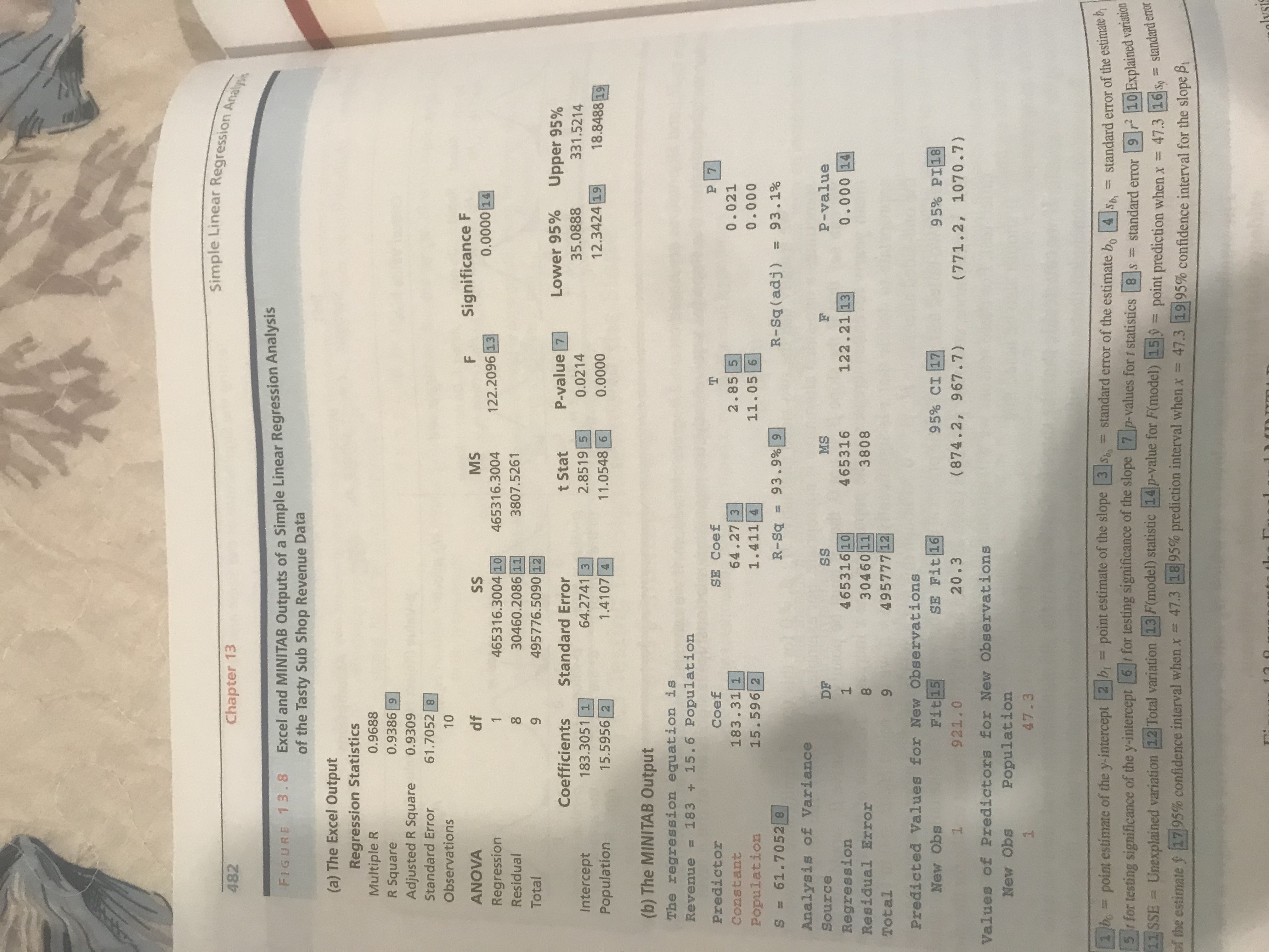
182 Chapter 13 Simple Linear Regression Analysis FIGURE 13. 8 Excel and MINITAB Outputs of a Simple Linear Regression Analysis of the Tasty Sub Shop Revenue Data (a) The Excel Output Regression Statistics Multiple R 0.9688 R Square 0.9386 9 Adjusted R Square 0.9309 Standard Error 61.7052 8 Observations 10 ANOVA MS F Significance F df SS 0.0000 14 Regression 465316.3004 10 465316.3004 122.2096 13 Residual 40 00- 30460.2086 11 3807.5261 Total 495776.5090 12 Coefficients Standard Error t Stat P-value 7 Lower 95% Upper 95% 183.3051 1 64.2741 3 2.8519 5 0.0214 35.0888 Intercept 331.5214 Population 15.5956 2 1.4107 4 11.0548 6 0.0000 12.3424 19 18.8488 19 (b) The MINITAB Output The regression equation is Revenue = 183 + 15.6 Population Predictor Coef SE Coef T P 7 Constant 183 . 31 1 64.27 3 2. 85 5 0 . 021 Population 15. 596 2 1. 411 4 11 .05 6 0 . 000 S = 61. 7052 8 R-Sq = 93. 9% 9 R-Sq (adj ) = 93.1% Analysis of Variance Source DF SS MS F P-value Regression 465316 10 465316 122. 21 13 0 . 000 14 Residual Error 10 0 H 30460 11 3808 Total 495777 12 Predicted Values for New Observations New Obs Fit 15 SE Fit 16 95% CI 17 95% PI 18 921.0 20 . 3 (874 .2, 967.7) (771.2, 1070.7) Values of Predictors for New Observations New Obs Population 47 .3 1 bo = point estimate of the y-intercept [2 b, = point estimate of the slope | 3 s, = standard error of the estimate bo [4 ]So, = standard error of the estimate 5 f for testing significance of the y-intercept 6 / for testing significance of the slope 7 p-values for t statistics 8 s = standard error 9 2 10 Explained variauo 11 SSE = Unexplained variation 12 Total variation 13 F(model) statistic 14 p-value for F(model) [15 9 = point prediction when x = 47.3 16)s, = standard en of the estimate $ 17 95% confidence interval when x = 47.3 18 95% prediction interval when x = 47.3 19 95% confidence interval for the slope By13.14 What do we conclude if we can reject Ho: B, = 0 in favor of Ha: B, # 0 by setting a a equal to .05? b a equal to . 01? 13.15 Give an example of a practical application of the confidence interval for B,. METHODS AND APPLICATIONS In Exercises 13.16 through 13.19, we refer to Excel and MINITAB outputs of simple linear regression analy- ses of the data sets related to the four case studies introduced in the exercises for Section 13.1. Using the appropriate output for each case study, a Find the least squares point estimates bo and b, of Bo and B, on the output and report their values. b Find SSE and s on the computer output and report their values.Chapter 13 Simple Linear Regression Analysis Find s , and the t statistic for testing the significance of the slope on the output and report their values Show (within rounding) how t has been calculated by using b, and s, from the computer output. d Using the t statistic and an appropriate critical value, test Ho: B, = 0 versus Ha: B, # 0 by setting a equal to .05. Is the slope (regression relationship) significant at the .05 level? e Using the t statistic and an appropriate critical value, test Ho: B1 = 0 versus Ha: B, # 0 by setting a equal to .01. Is the slope (regression relationship) significant at the .01 level? f Find the p-value for testing Ho: B, = 0 versus Ha: , # 0 on the output and report its value. Using the p-value, determine whether we can reject Ho by setting a equal to . 10, .05, .01, and .001. How much evidence is there that the slope (regression relationship) is significant? g Calculate the 95 percent confidence interval for , using numbers on the output. Interpret the interval. h Calculate the 99 percent confidence interval for B, using numbers on the output. i Find sp, and the t statistic for testing the significance of the y intercept on the output and report their val- ues. Show (within rounding) how t has been calculated by using bo and sb, from the computer output. j Find the p-value for testing Ho: Bo = 0 versus Ha: Bo # 0 on the computer output and report its value. Using the p-value, determine whether we can reject Ho by setting a equal to .10, .05, .01, and .001. What do you conclude about the significance of the y intercept? k Using the data set and s from the computer output, hand calculate (within rounding) SS, S, and so. AL GAS CONSUMPTION CASE DS GasCon1 d MINITAB outputs of a simple linear regression analysis of the data set for this case (see Exercise 13.3 on 1475) are given in Figures 13.9 and 13.10. Recall that labeled Excel and MINITAB outputs are on page 482 xcel Output of a Simple Linear Regression Analysis of the Natural Gas Consumption Data or Exercise 13.16)