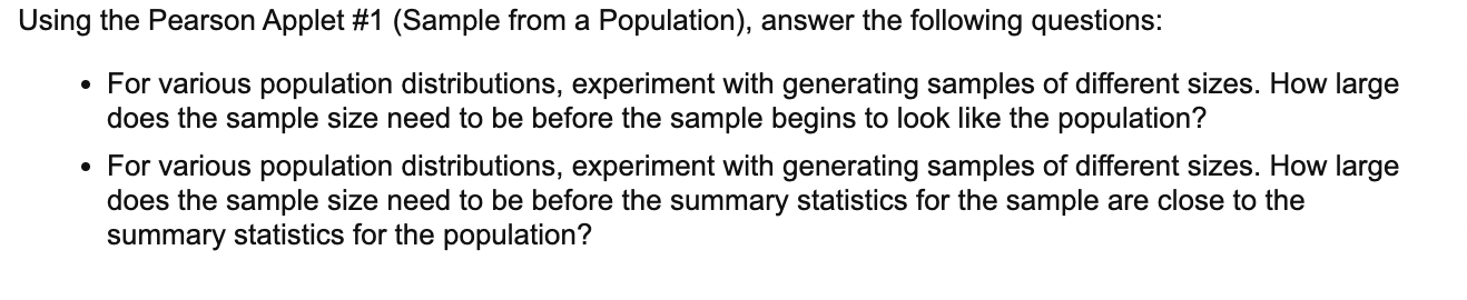
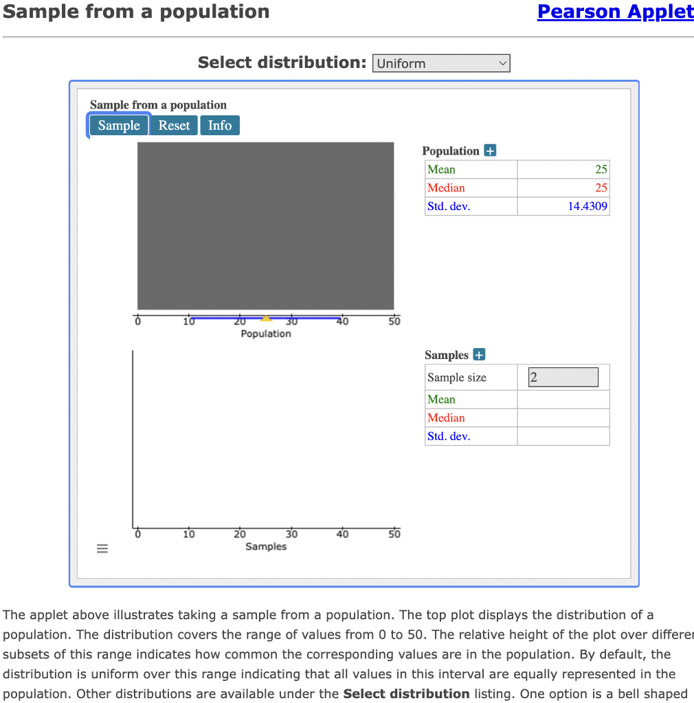
Using the Pearson Applet #1 (Sample from a Population), answer the following questions: For various population distributions, experiment with generating samples of different sizes. How large does the sample size need to be before the sample begins to look like the population? For various population distributions, experiment with generating samples of different sizes. How large does the sample size need to be before the summary statistics for the sample are close to the summary statistics for the population? Sample from a population Sample from a population Sample Reset Info 10 ZO Population 10 40 50 20 30 Samples The applet above illustrates taking a sample from a population. The top plot displays the distribution of a population. The distribution covers the range of values from 0 to 50. The relative height of the plot over differe subsets of this range indicates how common the corresponding values are in the population. By default, the distribution is uniform over this range indicating that all values in this interval are equally represented in the population. Other distributions are available under the Select distribution listing. One option is a bell shaped III = Select distribution: Uniform 30 40 50 Pearson Applet 25 25 14.4309 Population + Mean Median Std. dev. Samples + Sample size Mean Median Std. dev. 2 distribution centered on 25 where values between 20 and 30 are much more common in the population than values outside that range. Another option is a right skewed distribution where smaller values (below 20) are much more common than higher values (close to 50). There are also a number of options for creating a discrete distribution containing only the values of 0 and 1. The proportion of 1s in the population, denoted by p, can be specified from 0.1 to 0.9 in increments of 0.1. Lastly, a continuous custom distribution starting from a blank slate can also be created. The distribution can be changed interactively by clicking and dragging the mouse along the plot tracing out the shape of the desired distribution. When the Sample button is clicked, a random sample of size specified under Sample size within the Samples table will be selected from the population and displayed in the bottom plot. If the sample size is less than or equal to 30, the display will show the points randomly selected from the population dropping into the samples plot in an animated fashion. Summary statistics for the population and the sample are shown in the panel to the left of each plot. Using the Pearson Applet #1 (Sample from a Population), answer the following questions: For various population distributions, experiment with generating samples of different sizes. How large does the sample size need to be before the sample begins to look like the population? For various population distributions, experiment with generating samples of different sizes. How large does the sample size need to be before the summary statistics for the sample are close to the summary statistics for the population? Sample from a population Sample from a population Sample Reset Info 10 ZO Population 10 40 50 20 30 Samples The applet above illustrates taking a sample from a population. The top plot displays the distribution of a population. The distribution covers the range of values from 0 to 50. The relative height of the plot over differe subsets of this range indicates how common the corresponding values are in the population. By default, the distribution is uniform over this range indicating that all values in this interval are equally represented in the population. Other distributions are available under the Select distribution listing. One option is a bell shaped III = Select distribution: Uniform 30 40 50 Pearson Applet 25 25 14.4309 Population + Mean Median Std. dev. Samples + Sample size Mean Median Std. dev. 2 distribution centered on 25 where values between 20 and 30 are much more common in the population than values outside that range. Another option is a right skewed distribution where smaller values (below 20) are much more common than higher values (close to 50). There are also a number of options for creating a discrete distribution containing only the values of 0 and 1. The proportion of 1s in the population, denoted by p, can be specified from 0.1 to 0.9 in increments of 0.1. Lastly, a continuous custom distribution starting from a blank slate can also be created. The distribution can be changed interactively by clicking and dragging the mouse along the plot tracing out the shape of the desired distribution. When the Sample button is clicked, a random sample of size specified under Sample size within the Samples table will be selected from the population and displayed in the bottom plot. If the sample size is less than or equal to 30, the display will show the points randomly selected from the population dropping into the samples plot in an animated fashion. Summary statistics for the population and the sample are shown in the panel to the left of each plot