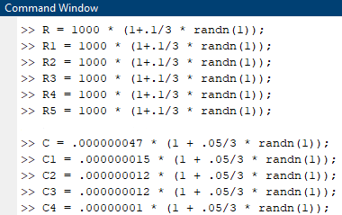
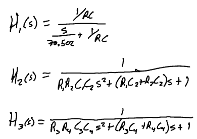
Values found: (IGNORE R5 as it is not necessary)

Transfer Function: 5th order broken down into 1, 1st order and 2, 2nd orders

QUESTION:

PLEASE HELP NEED MATLAB CODE AND PLOTS TO MAKE SENSE OF HOW TO DO THIS... THANK YOU!

ask for any more information needed and I will reply ASAP!

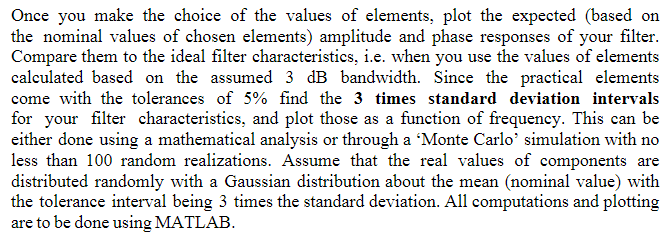
Command Window >> R = 1000 * (1+.1/3 * randn (1)); >> R1 = 1000 * (1+.1/3 * randn (1)); >> R2 = 1000 * (1+.1/3 * randn (1)); = >> R3 = 1000 * 1000 * (1+.1/3 * randn (1)); >> R4 = 1000 * (1+.1/3 * randn(1)); = >> R5 = 1000 * (1+.1/3 * randn(1)); = 3 >> C = .000000047 * (1 + .05/3 * randn (1)); >> C1 = .000000015 * (1 + .05/3 * randn (1)); >> C2 = .000000012 * (1 + .05/3 * randn(1)); >> C3 = .000000012 * (1 + .05/3 * randn (1)); >> C4 = .0000000l * .00000001 * (1 + .05/3 * randn (1)); = YRC H, (s) = I +YRC 70,502 2 H (s) = R,A,C,{5+ (B,C 272, (z)s +7 1 H36 H2A) = , 56,337 Gast 1 RR SC, s+(Rg Cu thy (a)s + 1 Once you make the choice of the values of elements, plot the expected (based on the nominal values of chosen elements) amplitude and phase responses of your filter. Compare them to the ideal filter characteristics, i.e. when you use the values of elements calculated based on the assumed 3 dB bandwidth. Since the practical elements come with the tolerances of 5% find the 3 times standard deviation intervals for your filter characteristics, and plot those as a function of frequency. This can be either done using a mathematical analysis or through a Monte Carlo simulation with no less than 100 random realizations. Assume that the real values of components are distributed randomly with a Gaussian distribution about the mean (nominal value) with the tolerance interval being 3 times the standard deviation. All computations and plotting are to be done using MATLAB. Command Window >> R = 1000 * (1+.1/3 * randn (1)); >> R1 = 1000 * (1+.1/3 * randn (1)); >> R2 = 1000 * (1+.1/3 * randn (1)); = >> R3 = 1000 * 1000 * (1+.1/3 * randn (1)); >> R4 = 1000 * (1+.1/3 * randn(1)); = >> R5 = 1000 * (1+.1/3 * randn(1)); = 3 >> C = .000000047 * (1 + .05/3 * randn (1)); >> C1 = .000000015 * (1 + .05/3 * randn (1)); >> C2 = .000000012 * (1 + .05/3 * randn(1)); >> C3 = .000000012 * (1 + .05/3 * randn (1)); >> C4 = .0000000l * .00000001 * (1 + .05/3 * randn (1)); = YRC H, (s) = I +YRC 70,502 2 H (s) = R,A,C,{5+ (B,C 272, (z)s +7 1 H36 H2A) = , 56,337 Gast 1 RR SC, s+(Rg Cu thy (a)s + 1 Once you make the choice of the values of elements, plot the expected (based on the nominal values of chosen elements) amplitude and phase responses of your filter. Compare them to the ideal filter characteristics, i.e. when you use the values of elements calculated based on the assumed 3 dB bandwidth. Since the practical elements come with the tolerances of 5% find the 3 times standard deviation intervals for your filter characteristics, and plot those as a function of frequency. This can be either done using a mathematical analysis or through a Monte Carlo simulation with no less than 100 random realizations. Assume that the real values of components are distributed randomly with a Gaussian distribution about the mean (nominal value) with the tolerance interval being 3 times the standard deviation. All computations and plotting are to be done using MATLAB