Visualization in python

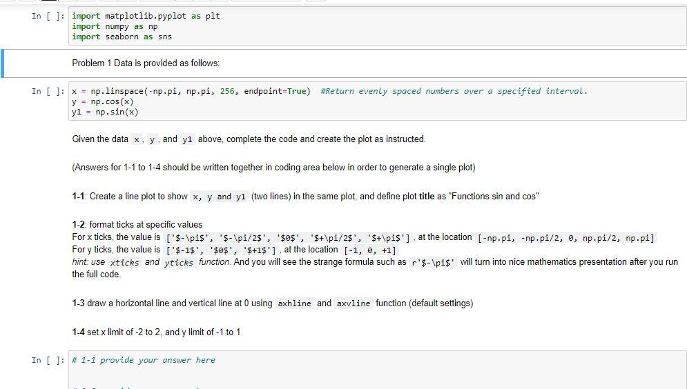
import matplotlib.pyplot as plt import numpy as np import seaborn as sns

x = np.linspace(-np.pi, np.pi, 256, endpoint=True) #Return evenly spaced numbers over a specified interval. y = np.cos(x) y1 = np.sin(x)

Given the data x, y, and y1 above, complete the code and create the plot as instructed.

(Answers for 1-1 to 1-4 should be written together in coding area below in order to generate a single plot)

1-1: Create a line plot to show x, y and y1 (two lines) in the same plot, and define plot title as "Functions sin and cos"

1-2: format ticks at specific values For x ticks, the value is ['$-\pi$', '$-\pi/2$', '$0$', '$+\pi/2$', '$+\pi$'], at the location [-np.pi, -np.pi/2, 0, np.pi/2, np.pi] For y ticks, the value is ['$-1$', '$0$', '$+1$'], at the location [-1, 0, +1] hint: use xticks and yticks function. And you will see the strange formula such as r'$-\pi$' will turn into nice mathematics presentation after you run the full code.

1-3 draw a horizontal line and vertical line at 0 using axhline and axvline function (default settings)

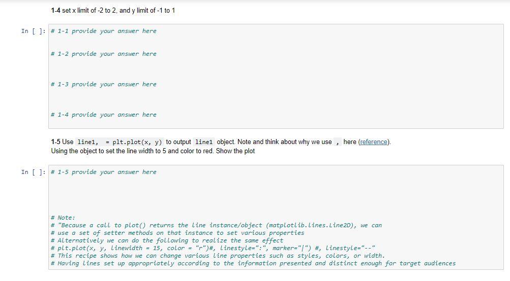
1-4 set x limit of -2 to 2, and y limit of -1 to 1

1-5 Use line1, = plt.plot(x, y) to output line1 object. Note and think about why we use , here (reference). Using the object to set the line width to 5 and color to red. Show the plot

Problem 2 Iris Data Analysis

Q2-

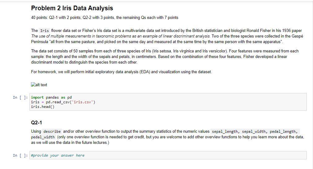
The Iris flower data set or Fisher's Iris data set is a multivariate data set introduced by the British statistician and biologist Ronald Fisher in his 1936 paper The use of multiple measurements in taxonomic problems as an example of linear discriminant analysis. Two of the three species were collected in the Gasp Peninsula "all from the same pasture, and picked on the same day and measured at the same time by the same person with the same apparatus".

The data set consists of 50 samples from each of three species of Iris (Iris setosa, Iris virginica and Iris versicolor). Four features were measured from each sample: the length and the width of the sepals and petals, in centimeters. Based on the combination of these four features, Fisher developed a linear discriminant model to distinguish the species from each other.

For homework, we will perform initial exploratory data analysis (EDA) and visualization using the dataset.

import pandas as pd iris = pd.read_csv('iris.csv') iris.head()

Q2-1

Using describe and/or other overview function to output the summary statistics of the numeric values sepal_length, sepal_width, pedal_length, pedal_width (only one overview function is needed to get credit, but you are welcome to add other overview functions to help you learn more about the data, as we will use the data in the future lectures.)

Q2-2

It will be interesting to see if the numeric values sepal_length, sepal_width, pedal_length, pedal_width has any kind of relationships among them. Looking at the correlation among the variables is normally a good start for getting insights of the data/fields.

For homework exercise, use the corr and sns.heatmap function (taught in class) to plot the correlation heatmap among the four numeric variables. Your output figures should be similar to attached iris_corr.png file.

In [ ] : # provide your answer here

As is expected, there is a strong correlation between pedal_length, pedal_width (=0.96=0.96). However, the relationship between the sepal_length, sepal_width is not so clear (=0.11=0.11).

Given the above information, seems the relationship between sepal_length, sepal_width is not so clear, let's try more charting methodologies to see if there is any clue (as learning experience, some types of charts may not work well)

Q2-3 Line Chart:

Plot line chart for sepal_length and sepal_width columns. One line for each column. Show the legends to distinguish which line stands for. Your output figures should be similar to attached line_chart.png file.

In [ ] : # provide your answer here

Seems line chart does not offer a lot of clues. We may want to switch to different charts.

Q2-4 Histogram:

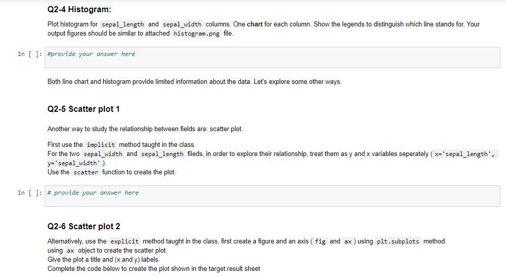
Plot histogram for sepal_length and sepal_width columns. One chart for each column. Show the legends to distinguish which line stands for. Your output figures should be similar to attached histogram.png file.

In [ ] : # provide your answer here

Both line chart and histogram provide limited information about the data. Let's explore some other ways.

Q2-5 Scatter plot 1

Another way to study the relationship between fields are: scatter plot.

First use the implicit method taught in the class. For the two sepal_width and sepal_length fileds, in order to explore their relationship, treat them as y and x variables seperately (x='sepal_length', y='sepal_width'). Use the scatter function to create the plot.

In [ ] : # provide your answer here

Q2-6 Scatter plot 2

Alternatively, use the explicit method taught in the class, first create a figure and an axis (fig and ax) using plt.subplots method. using ax object to create the scatter plot. Give the plot a title and (x and y) labels. Complete the code below to create the plot shown in the target result sheet

In [ ] :

# create a figure and axis fig, ax = plt.subplots()

# scatter the sepal_length against the sepal_width # provide your answer here

# set a title # provide your answer here # set x labels # provide your answer here # set y labels # provide your answer here

The relationship is still not clear. Let's keep digging. Iris has three types, 'Iris-setosa', 'Iris-versicolor' and 'Iris-virginica'. Next we will label the above dot in the charts with three differernt colors to distinguish the three types in the above scatter chat (may consider using explicit method and for loop, but you do not have to. Feel free to create new codes), and see if there is change in the observed relationship. hint: you may choose to use color = colors[iris['class'][i]] in your scatter plot settings, in order to leveraging colors = {'Iris-setosa':'r', 'Iris-versicolor':'g', 'Iris-virginica':'b'}

In [ ] :

# create color dictionary, for example Setosa will be labeled red colors = {'Iris-setosa':'r', 'Iris-versicolor':'g', 'Iris-virginica':'b'} # create a figure and axis fig, ax = plt.subplots() # plot each data-point using three different colors for i in range(len(iris['sepal_length'])): # provide your answer here # set a title # provide your answer here # set x labels # provide your answer here # set y labels # provide your answer here

In [ ]; import matplotlib.pyplot as plt import numpy as np import seaborn as sns Problem 1 Data is provided as follows: In [ ]: x = np.linspace(-np.pi, np.pi, 256, endpoint=True) #Return evenly spaced numbers over a specified interval. y = np.cos(x) y1 = np.sin(x) Given the data x, y, and y1 above, complete the code and create the plot as instructed. (Answers for 1-1 to 1-4 should be written together in coding area below in order to generate a single plot) 1-1: Create a line plot to show x, y and yi (two lines) in the same plot, and define plot title as "Functions sin and cos" 1-2: format ticks at specific values For x ticks, the value is ['$-\pis', '$-\pi/2$', '$0$', '$+\pi/2$', '$+\pis'], at the location [-np.pi, -np.pi/2, 0, np.pi/2, np.pi] For y ticks, the value is ['$-1$', '$0$', '$+1$'], at the location (-1, 0, +1] hint use xticks and yticks function. And you will see the strange formula such as r'$-\pis' will turn into nice mathematics presentation after you run the full code 1-3 draw a horizontal line and vertical line at 0 using axhline and axvline function (default settings) 1-4 set x limit of -2 to 2, and y limit of -1 to 1 In [ ]: # 1-1 provide your answer here 1-4 set x limit of -2 to 2. and y limit of -1 to 1 In [ ]: # 1-1 provide your answer here # 1-2 provide your answer here # 1-3 provide your answer here # 1-4 provide your answer here 1-5 Use linel, = plt.plot(x, y) to output linel object. Note and think about why we use, here (reference). Using the object to set the line width to 5 and color to red. Show the plot In [ ]: # 1-5 provide your ansiver here # Note: # "Because a call to plot() returns the line instance/object matplotlib.Lines. Line 2D), we can # use a set of setter methods on that instance to set various properties # Alternatively we can do the following to realize the same effect #plt.plot(x, y, Linewidth = 15, color = "r")#, Linestyle=":", marker="/") #, Linestyle="--" # This recipe shows how we can change various line properties such as styles, colors, or width. # Having Lines set up appropriately according to the information presented and distinct enough for target audiences Problem 2 Iris Data Analysis 40 points: Q2-1 with 2 points: Q2-2 with 3 points, the remaining Qs each with 7 points The Iris flower data set or Fisher's Iris data set is a multivariate data set introduced by the British statistician and biologist Ronald Fisher in his 1936 paper The use of multiple measurements in taxonomic problems as an example of linear discriminant analysis. Two of the three species were collected in the Gasp Peninsula "all from the same pasture, and picked on the same day and measured at the same time by the same person with the same apparatus". The data set consists of 50 samples from each of three species of Iris (Iris setosa, Iris virginica and Iris versicolor). Four features were measured from each sample: the length and the width of the sepals and petals, in centimeters. Based on the combination of these four features, Fisher developed a linear discriminant model to distinguish the species from each other. For homework, we will perform initial exploratory data analysis (EDA) and visualization using the dataset. alt text In [ ]: import pandas as pd iris = pd.read_csv('iris.csv') iris.head() Q2-1 Using describe and/or other overview function to output the summary statistics of the numeric values sepal_length, sepal_width, pedal_length, pedal_width (only one overview function is needed to get credit, but you are welcome to add other overview functions to help you learn more about the data, as we will use the data in the future lectures.) In [ ]: #provide your answer here Q2-4 Histogram: Plot histogram for sepal_length and sepal_width columns. One chart for each column. Show the legends to distinguish which line stands for. Your output figures should be similar to attached histogram.png file. In [ ]: #provide your answer here Both line chart and histogram provide limited information about the data. Let's explore some other ways. Q2-5 Scatter plot 1 Another way to study the relationship between fields are: scatter plot. First use the implicit method taught in the class. For the two sepal_width and sepal_length fileds, in order to explore their relationship, treat them as y and x variables seperately ( x='sepal_length', y='sepal_width'). Use the scatter function to create the plot. In [ ]: # provide your answer here Q2-6 Scatter plot 2 Alternatively, use the explicit method taught in the class, first create a figure and an axis ( fig and ax ) using plt.subplots method. using ax object to create the scatter plot. Give the plot a title and (x and y) labels. Complete the code below to create the plot shown in the target result sheet In [ ]: # create a figure and axis fig, ax = pit.subplotso) # scatter the sepol_Length against the sepal_width # provide your answer here # set a title # provide your answer here # set x Labels # provide your answer here # set y Labels # provide your answer here Q2-7 Scatter plot 3 The relationship is still not clear. Let's keep digging Iris has three types, 'Iris-setosa', 'Iris-versicolor' and 'Iris-virginica'. Next we will label the above dot in the charts with three differernt colors to distinguish the three types in the above scatter chat (may consider using explicit method and for loop, but you do not have to. Feel free to create new codes) and see if there is change in the observed relationship hint you may choose to use color = colors[iris['class'][i]] in your scatter plot settings, in order to leveraging colors = {'Iris-setosa':'r', 'Iris-versicolor':'g', 'Iris-virginica': 'b'} In [ ]: # create color dictionary, for example setosa will be Labeled red colors = {'Iris-setosa':'r', 'Iris-versicolor':'g', 'Iris-virginica': 'b'} # create a figure and axis fig, ax = pit. subplots() #plot each dota-point using three different colors for i in range(len(iris['sepal_length'])): # provide your answer here # set a title # provide your answer here # set x Labels # provide your answer here # set y Labels # provide your answer here